We compare the state-covariance-based high resolution tools with the MUSIC and ESPRIT methods for spectral line detection. We consider a real-valued time series which is an additive composition of

sinusoids with white noise. The length of observation record is N=1000

, and

where

and

. The noise is white, Gaussian, with standard deviation 0.35

. For each observation record, we estimate spectral lines using MUSIC, ESPRIT and the state-covariance-based methods. We compare the results from 100

runs.

% demo: scatter plots comparing sm with music and esprit
%       it shows that the variance of the sm-estimates is
%       superior to the other two.
%
% simulation example from sesha2 page 38

% Setting up the signal parameters and time interval
% here y=unit variance white noise + .5*sin(.1*t+phi1) + sin(.15*t+phi2)
clear, close all

N=1000; mag0=.35; mag1=.5; o1=.1; mag2=1; o2=.15;
t=0:N-1; t=t(:);

% drawing the target frequency1 vs frequency2 for the subsequently generated
% scatter diagrams
figure(1), clf,
subplot(3,1,1), plot(o1,o2,'rx','MarkerSize',12),  hold on,
subplot(3,1,2), plot(o1,o2,'rx','MarkerSize',12),  hold on,
subplot(3,1,3), plot(o1,o2,'rx','MarkerSize',12),  hold on,


% simulating the time series and determining the frequencies of the two
% sinusoids.
IS_count=0;
MUSIC_count=0;
ESPRIT_count=0;
for i=1:100,
  y=mag0*randn(N,1)+mag1*sin(o1*t+2*pi*rand)+mag2*sin(o2*t+2*pi*rand);

% estimating sinusoids per music, esprit
n=4; m=30;
omusic=music(y,n,m); omusic=omusic(omusic>=0);
omusic=sort(omusic); omusic=omusic(end-1:end);
oesprit=esprit(y,n,m); oesprit=oesprit(oesprit>=0);
oesprit=sort(oesprit); oesprit=oesprit(end-1:end);

% IS-based estimation
thetamid=.05; [Ah,bh]=cjordan([30],[0.4*exp(thetamid*j)]);

P=dlsim_complex(Ah,bh,y');

[omega_ss,residues_ss]=sm(P,Ah,bh,n);
omega_ss=omega_ss(omega_ss<pi);
omega_ss=sort(omega_ss);omega_ss=omega_ss(end-1:end);

if(omega_ss(1)>0.07&&omega_ss(1)<0.13&&omega_ss(2)>0.12&&omega_ss(2)<0.18)
    IS_count=IS_count+1;
end
if(omusic(1)>0.07&&omusic(1)<0.13&&omusic(2)>0.12&&omusic(2)<0.18)
    MUSIC_count=MUSIC_count+1;
end
if(oesprit(1)>0.07&&oesprit(1)<0.13&&oesprit(2)>0.12&&oesprit(2)<0.18)
    ESPRIT_count=ESPRIT_count+1;
end

% [omega_ss,omusic oesprit];
subplot(3,1,1), plot(omega_ss(1),omega_ss(2),'o'),
subplot(3,1,2), plot(omusic(1),omusic(2),'o'),
subplot(3,1,3), plot(oesprit(1),oesprit(2),'o'),
end

figure(1),
subplot(3,1,1), axis([.07 .13 .12 .18]); hold on,  legend('sm')
subplot(3,1,2), axis([.07 .13 .12 .18]); hold on,  legend('music')
subplot(3,1,3), axis([.07 .13 .12 .18]); hold on,  legend('esprit')

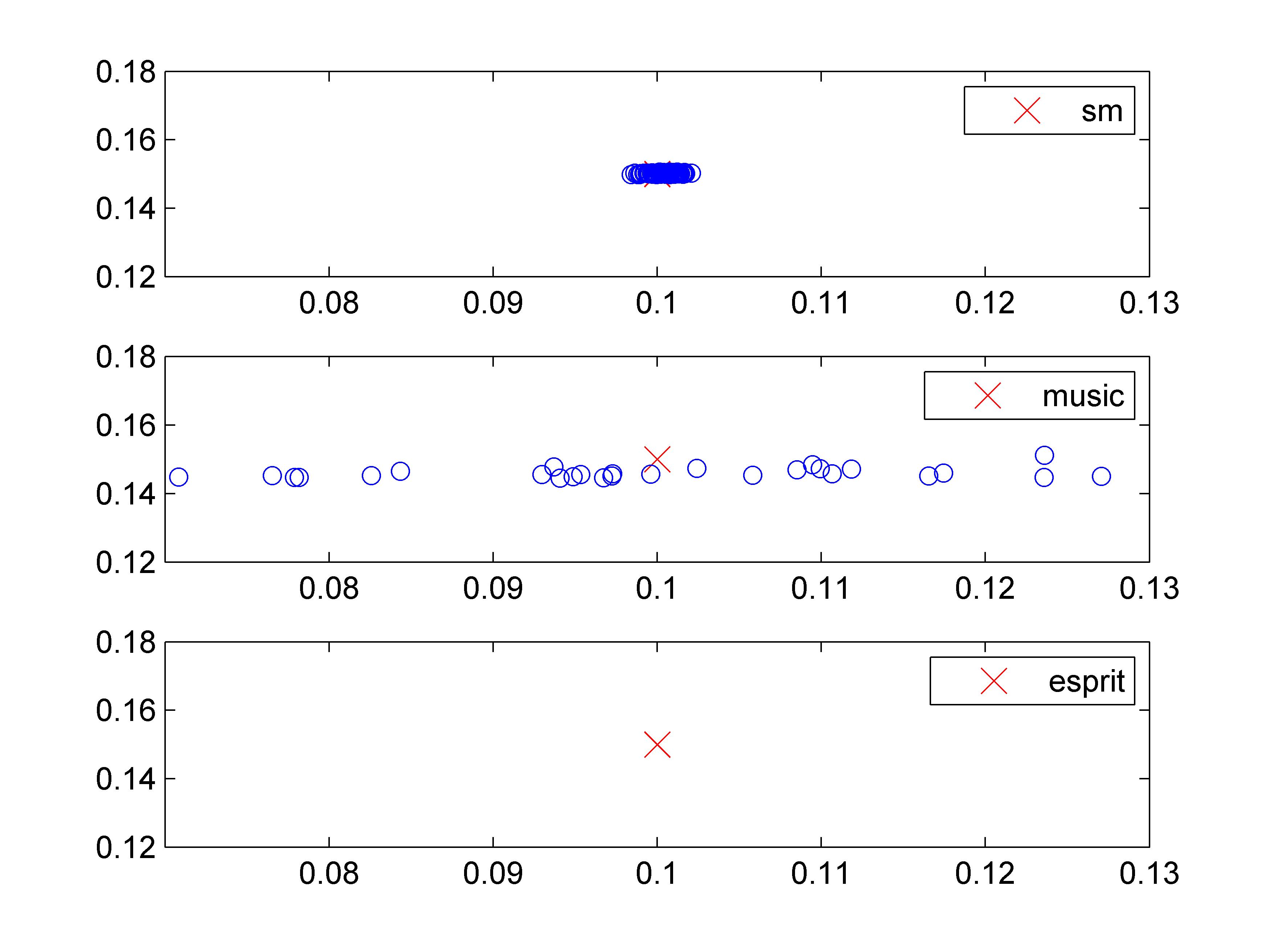
We display below the scatter plots of the estimated theta_1

v.s.

. The red cross marks the target frequencies. We choose a small window containing the target and if there is point detected inside the box, we claim a detection. There are totally 100

detections for the state-covariance-based method (100% success) and

detections for the MUSIC method, and none for the ESPRIT method. We also see that the results given by the state-covariance-based method are very concentrated around the target point.

Comparison with MUSIC and ESPRIT