% setting up filter parameters and the svd of the input-to-state response
thetamid=1.325;
[A,B]=cjordan(5,0.88*exp(thetamid*1i));
% obtaining state statistics
R=dlsim_complex(A,B,y');
sv=Rsigma(A,B,th);
plot(th(:),sv(:));
Input-to-state filter and state covariance
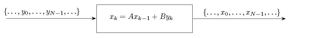
The first step to explain the high resolution spectral analysis tools is to consider the input-to-state
filter below and the corresponding
the state statistics.
The process  is the input and
  is the state.
 |
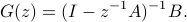
Then the filter transfer function is
A positive semi-definite matrix  is the state covariance of the above filter, i.e.
 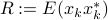 for some stationary input
process
for some stationary input
process  , if and only if it satisfies the following
equation
, if and only if it satisfies the following
equation

for some row-vector  .
Starting from a finite number of samples, we denote
.
Starting from a finite number of samples, we denote
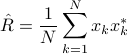
the sample state covariance matrix.
If the matrix  is the companion matrix
![A = left[ begin{array}{ccccc} 0 & 0 & ldots & 0 & 0 1 & 0 & ldots & 0 & 0 vdots & vdots & & vdots& vdots 0 & 0 & ldots & 1 & 0 end{array} right], ~~ B= left[ begin{array}{c} 1 0 vdots 0 end{array} right], hspace*{3cm} (1)](eqs/720422545-130.png)
the filter is a tapped delay line:
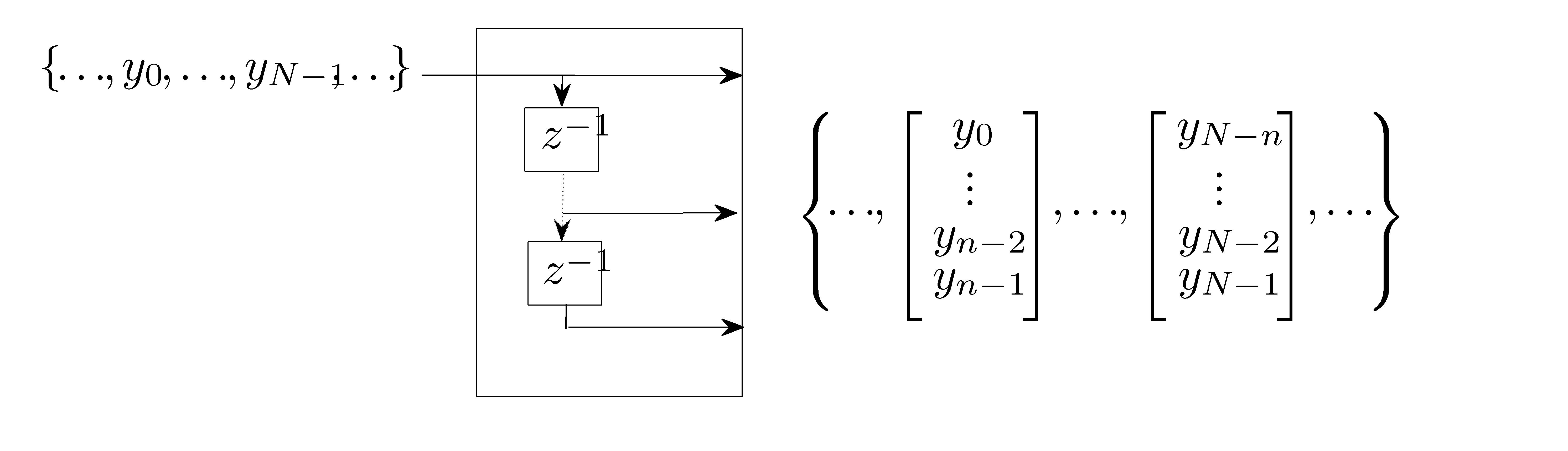 |
The corresponding state covariance is Toeplitz matrix. Thus the state-covariance formalism subsumes the theory of Toeplitz matrices.
The input-to-state filter works as a “magnifying glass” or, as type of bandpass filter, amplifying the harmonics in a particular frequency interval.
Shaping of the filter is accomplished via selection of the eigenvalues of . In the above example, we set  eigenvalues of at
  , and the phase
angle
, and the phase
angle  is the middle of the interval
 ![[theta_1,;theta_2]](eqs/922774589-130.png) where resolution is desirable. Then we build the pair
where resolution is desirable. Then we build the pair  using routine cjordan.m, (and rjordan.m for real valued
problem).
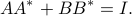
The pair is normalized to satisfy
using routine cjordan.m, (and rjordan.m for real valued
problem).
The pair is normalized to satisfy
The routine dlsim_complex.m generate the state covariance matrix (dlsim_real.m for
real valued problem).
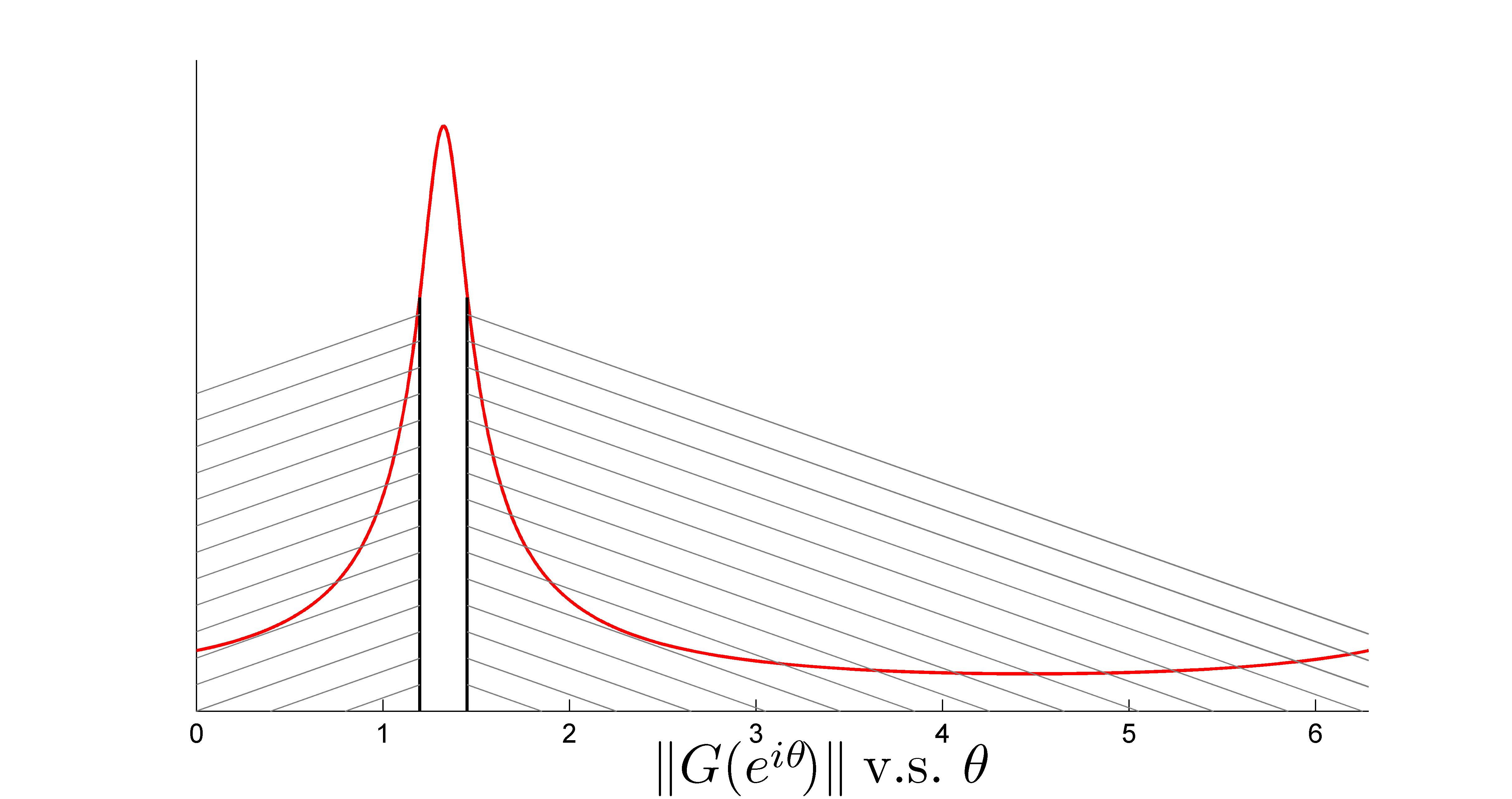
The following figure plots  versus
  . The gain
at equal
. The gain
at equal  and
and  is approximately
  dB below peak value. The window is marked in the following figure. The figure to the right shows the detail within the window of interest.
 |