Geometric methods for the estimation of structured covariances
 |
Introduction
Consider a zero-mean, real-valued, discrete-time, stationary random process  . Let
. Let

denote the autocorrelation function, and
![T:= left[ begin{array}{cccc} r(0) & r(1) & ldots& r(n-1) r(-1)& r(0) & ldots & r(n-2) vdots& vdots & ddots & vdots r(-n+1)& r(-n+2)& ddots& r(0) end{array}right]](eqs/946992604-130.png)
the covariance of the finite observation vector
![{{bf x}} = [x(0),~ x(1),~ldots,~x(n-1)]'](eqs/1063528008-130.png)
i.e.  . Estimating
  from an observation record is often the first step in spectral analysis.
 |
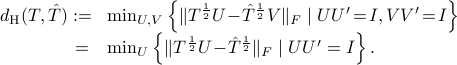
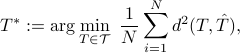
may not have the Toeplitz structure. We seek a Toeplitz structured estimate by solving
where  . In this,
  represents a suitable notion of distance.
In the following, we overview some notions of distance and the relation among them. If the distance is not symmetric, we use
represents a suitable notion of distance.
In the following, we overview some notions of distance and the relation among them. If the distance is not symmetric, we use  instead. This approach can be carried out verbatim in approximating state covariances.
Likelihood divergence
Assuming that  is Gaussian, and letting
 ![{bf x}:= [{bf x}_1,ldots, {bf x}_m]](eqs/1114427224-130.png) , the joint density function is
, the joint density function is

where  is the sample covariance matrix.
Given
is the sample covariance matrix.
Given  , it is natural to seek a
  such that
  , equivalently
  , is maximal.
Alternatively, one may consider the likelihood divergence
, is maximal.
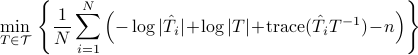
Alternatively, one may consider the likelihood divergence
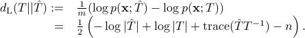
Using  , then the relevant optimization problem in
  is
is

which is not convex. A necessary condition for a local minimum is given in [Burg, et al.]:
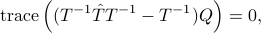
for all Toeplitz  . An iterative algorithm for solving the above equation and obtain a (local) minimum is proposed in [Burg, et al.]. This is implemented in CovEst_blw.m.
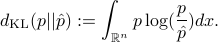
Kullback-Leibler divergence
The Kullback-Leibler (KL) divergence between two probability density functions  ,
,  on
on  is
is
In the case where and are normal with zero-mean and covariance and , respectively, their KL divergence becomes

while switching the order 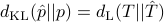 given earlier.
If
given earlier.
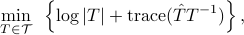
If  is used in , then the optimization problem becomes
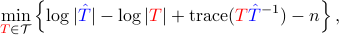
which is convex. This is implemented in CovEst_KL.m which requires the installation of cvx.
Fisher metric and geodesic distance
The KL divergence induces the Fisher metric, which is the quadratic term of 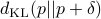
For probability distributions parameterized by a vector  , the corresponding metric is often referred to as the
Fisher-Rao metric and given by
, the corresponding metric is often referred to as the
Fisher-Rao metric and given by
![g_{p,{rm Fisher-Rao}}(delta_theta)=delta_{theta}'Eleft[ left( frac{partial log p}{partialtheta}right)left( frac{partial log p}{partialtheta}right)' right]delta_{theta}.](eqs/618555378-130.png)
For zero-mean Gaussian distributions parametrized by the corresponding covariance matrices, it becomes the Rao metric
The geodesic distance between two points and is the log-deviation distance

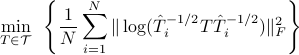
When  is used in , the corresponding optimization problem is not convex. Linearization of the objective function about
may be used instead, this leads to
is used in , the corresponding optimization problem is not convex. Linearization of the objective function about
may be used instead, this leads to
which is convex.
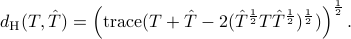
Bures metric and Hellinger distance
The Fisher information metric is the unique Riemannian metric for which stochastic maps are contractive [N. Cencov, 1982]. In quantum mechanics, a similar property has been sought for density matrices, which are positive semi-definite matrices with trace equal to one. There are several metrics for which stochastic maps are contractive. They take the form
For example, in the Bures metric

The Bures metric can also be written as

If  , we regard
  as a point on the unit sphere, and this point is not unique. The geodesic distance between two
density matrices is the smallest great-circle distance between corresponding points, which is call Bures length.
The smallest “straight line” distance is the Hellinger distance which is
as a point on the unit sphere, and this point is not unique. The geodesic distance between two
density matrices is the smallest great-circle distance between corresponding points, which is call Bures length.
The smallest “straight line” distance is the Hellinger distance which is
The distance has a closed form
When the above distance is used in , the corresponding optimization problem is
actually equivalent to a linear matrix inequality (LMI) [1]. This will be shown in the following section.
Transportation distance
Let  and
and  be random variables in
  having pdf's
  and
and  . A formulation of the Monge-Kantorovich
transportation problem (with a quadratic cost) is as follows. Determine
. A formulation of the Monge-Kantorovich
transportation problem (with a quadratic cost) is as follows. Determine
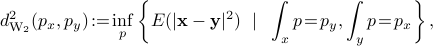
where is the joint distribution for and . The metric  is known as the Wasserstein metric. For and
being zero-mean normal with covariances and and also jointly normal, we obtain
is known as the Wasserstein metric. For and
being zero-mean normal with covariances and and also jointly normal, we obtain
![d^2_{rm{W_2}}(p, hat{p})= min_{S}left{ {rm trace}(T+hat{T}-S-S') ~mid~ left[ begin{array}{cc} T & S S' & hat{T} end{array} right]geq 0 right},](eqs/1916508557-130.png)
where  . The distance
  has a closed form
which is given by
has a closed form
which is given by
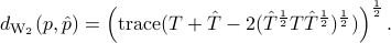
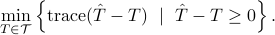
So  . So using either , or
  , the relevant optimization problem
becomes
, the relevant optimization problem
becomes
![min_{{color{red}T}in mathcal{T},; S}left{{rm trace}({color{red}T}+{color{blue}hat{T}}-S-S') ~mid~ left[ begin{array}{cc} {color{red}T} & S S' & {color{blue}hat{T}} end{array} right]geq 0right}.](eqs/588205696-130.png)
It is an LMI thus a convex optimization problem. This is implemented in CovEst_transp.m.
An alternative interpretation for the transportation distance is as follows. We postulate the stochastic model

where  represents noise, and and the covariances of
  and , respectively. By seeking the least possible noise variance while allowing possible coupling between and brings us the minimum transportation distance. Analogous rationale, albeit with different assumptions has been used to justify different methods. For instance, assuming that
  while and are independent leads to
This is implemented in CovEst_Q.m (SCovEst_Q.m for state-covariance estimation). Then, also, assuming a “symmetric” noise contribution as in
where the noise vectors  and are independent of and
  , we are called to solve

where  and designate covariances of and , respectively.
This is implemented in CovEst_QQh.m (SCovEst_QQh.m for state covariance estimation).
and designate covariances of and , respectively.
This is implemented in CovEst_QQh.m (SCovEst_QQh.m for state covariance estimation).
Mean-based covariance approximation
We investigate the concept of the mean as a way to fuse together sampled statistics from different sources into a structured one. In particular, given a set of
positive semi-definite matrices  , we consider the mean-based structured covariance
for a metric  or a divergence (and a suitable choice of power). Below, we consider each of the distances mentioned earlier.
Mean-based on KL divergence and likelihood
The optimization problem based on  is
is
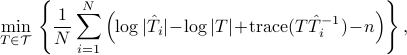
and is equivalent to
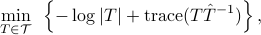
where 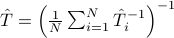 is the harmonic mean of the
  's.
On the other hand, if the likelihood divergence
's.
On the other hand, if the likelihood divergence  is used, the optimization problem
is equivalent to
where 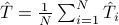 is the arithmetic mean of 's.
Mean based on log-deviation
In this case
is not convex in . If the admissible set  is relaxed to the set of positive definite matrices, the minimizer is precisely the geometric mean,
and it is the unique positive definite solution to the following equation
is relaxed to the set of positive definite matrices, the minimizer is precisely the geometric mean,
and it is the unique positive definite solution to the following equation
When  , is the unique geometric mean between two positive definite matrices
One may consider instead the linearized optimization problem
which is convex in .
Mean based on transportation/Bures/Hellinger distance
Using the transportation/Bures/Hellinger distance, the optimization problem becomes
![min_{Tin mathcal{T},; S_i}~bigg{frac{1}{N}sum_{i=1}^N{rm trace}(T+hat{T}_i-S_i-S_i') ~mid ~ left[ begin{array}{cc} T & S_i S_i' & hat{T}_i end{array} right]geq 0,~forall~ i=1,cdots, N bigg}.](eqs/576215841-130.png)
When is only constrained to be positive semi-definite, it has been shown that the transportation mean is the unique solution of the following equation
The routine Tmean.m provides a solution to the mean based Toeplitz estimation problem which is based on cvx
Examples
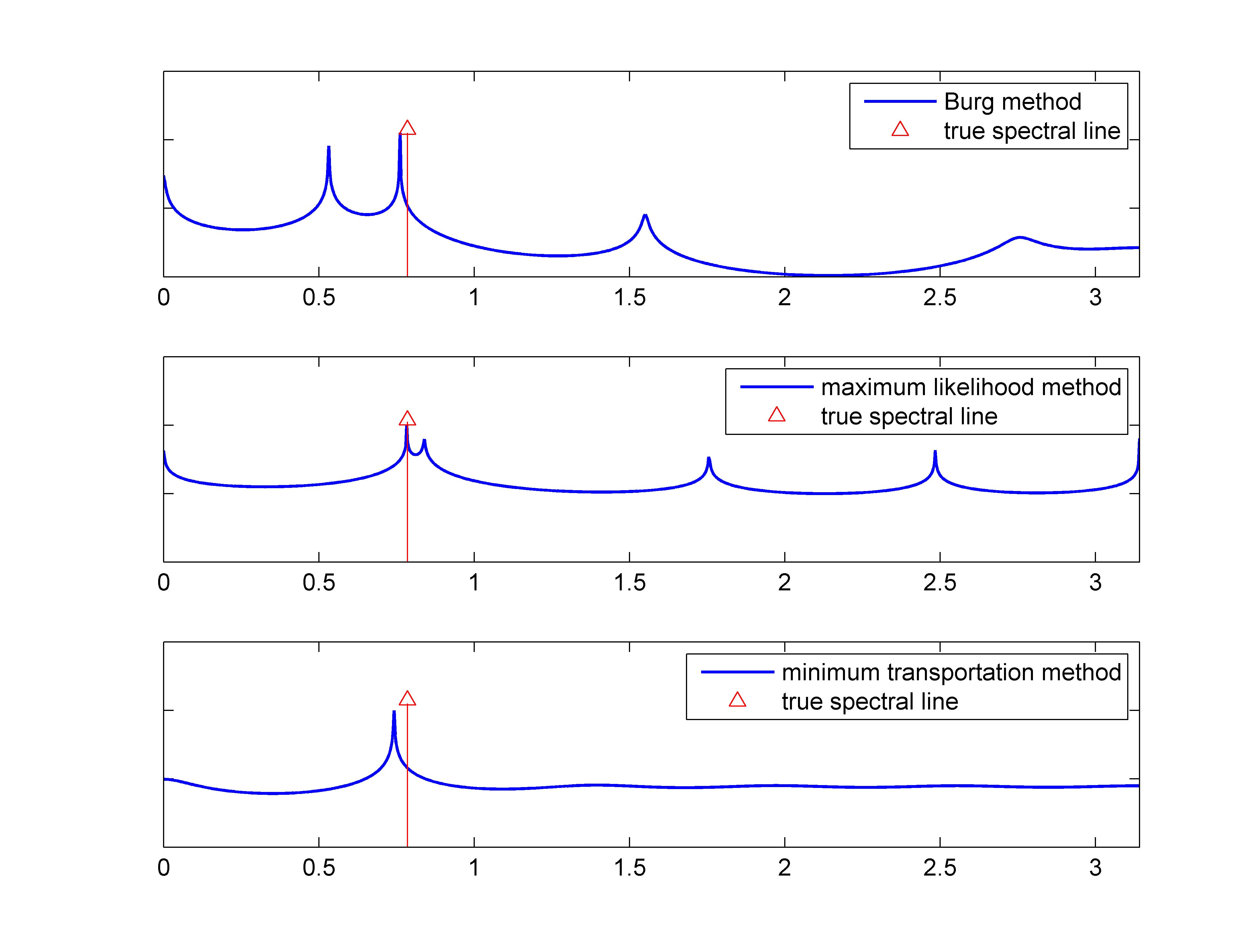
Identifying a spectral line in noise
We compare the performance of the likelihood estimation and the transportation-based method in identifying a single spectral line in white noise. Consider a single “observation record”

with the “noise”  generated from a zero-mean Gaussian distribution.
Hence the covariance matrix
generated from a zero-mean Gaussian distribution.
Hence the covariance matrix
![hat{T}=left[ begin{array}{c} x(0)x(1) vdots x(10)end{array}right]left[ begin{array}{cccc} x(0)&x(1)& cdots& x(10)end{array}right]](eqs/839213254-130.png)
is  and of rank equal to
  .
We use CovEst_blw and CovEst_transp to approximate with a covariance having admissible structure. We compare the corresponding maximum-entropy spectral estimates (subplot 2&3) with the spectrum obtained using pburg (matlab command) shown in subplot 1. The true spectral line is marked by an arrow in each plot.
.
We use CovEst_blw and CovEst_transp to approximate with a covariance having admissible structure. We compare the corresponding maximum-entropy spectral estimates (subplot 2&3) with the spectrum obtained using pburg (matlab command) shown in subplot 1. The true spectral line is marked by an arrow in each plot.
 |
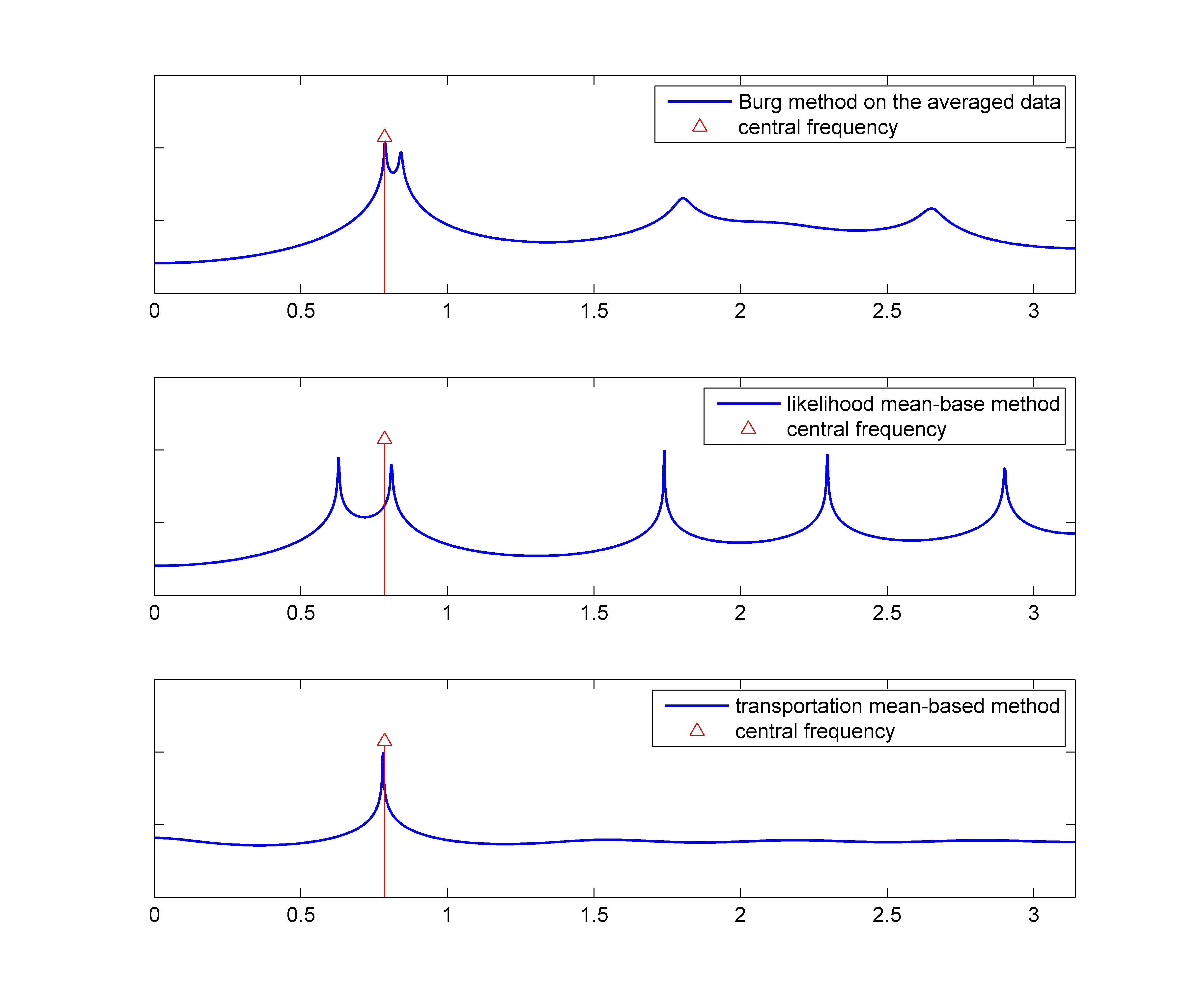
Averaging multiple spectra
Consider  different runs

with 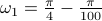 ,
,  ,
, 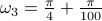 and
and  ,
,  ,
,  an
an  and
and  generated from zero-mean Gaussian distribution with variance
  . We consider the three rank one sample covariances. We estimate the likelihood and transportation mean of these three sampled covariance with the requirement that the mean also be Toeplitz (using CovEst_blw and Tmean). We plot the corresponding maximum entropy spectra. As a comparison, we also take the average of three observation records, and compute the Burg's spectrum based on the averaged data. The three results are shown in the following figure. Both the likelihood and the Burg's methods have two peaks near the central frequency
  , whereas the transportation-based method has only one peak at approximately the mean of the three instantiations of the underlying sinusoid.
 |
Reference
[1] L. Ning, X. Jiang and T.T. Georgiou, “Geometric methods for the estimation of structured covariances,” submitted, http://arxiv.org/abs/1110.3695.