%  SIGNAL = sinusoids + noise
%  Setting up the signal parameters and time history
N=100; n=15;
a0=1; a1=1.5; theta1=1.3; a2=2; theta2=1.35;
k=1:N; k=k(:);
y=a1*exp(1i*(theta1*k+2*pi*rand))+a2*exp(1i*(theta2*k+2*pi*rand));
% MA coefficient vector
b=[1.0000    0.4318   -0.4496   -0.5440];
u_real=randn(1,N+length(b)-1);
u_imag=randn(1,N+length(b)-1);
u=a0*(u_real+i*u_imag)/sqrt(2);
% generate noise
noise=b*toeplitz(u(length(b):-1:1),u(length(b):end));
y=y'+noise;
Ac=compan(eye(1,n+1));
Bc=eye(n,1);
That=dlsim_complex(Ac,Bc,y);
NN=2048; th=linspace(0,2*pi,NN);
T=ToepProj(That);
[Ts, Tma]=MA_decomp(T,3);
figure(1);clf
h=freqresp(f,th);
        subplot(3,1,1);
        plot(theta1,a1,'r^','MarkerSize',12);hold on;
        plot(th,vec(abs(h)).^2,'b','LineWidth',1.2);
        legend('true spectral line','true MA spectrum','Location','North');
        arrow([theta1 theta2],[a1 a2],12);
        set(gca,'xlim',[0 2*pi]);
        set(gca,'YTick',[]);


r_ma=[fliplr(Tma(1,:)) Tma(1,2:end)];
p_ma=abs(fft(r_ma,length(th)));
[w_s,r_s]=sm(Ts,Ac,Bc,rank(Ts,0.001));
r_s=r_s(w_s<pi); w_s=w_s(w_s<pi);
subplot(3,1,2);
        plot(w_s(1),r_s(1),'r^','MarkerSize',12);hold on;
        plot(th,p_ma,'b','LineWidth',1.2);
        legend('estimated spectral line','estimated MA spectrum','Location','North');
        arrow(w_s,r_s,12);
        set(gca,'xlim',[0 2*pi]);
        set(gca,'YTick',[]);


[Ts0, Tn]=MA_decomp(T,0);
[w_s0,r_s0]=sm(Ts0,Ac,Bc,rank(Ts0,0.001));
r_s0=r_s0(w_s0<pi); w_s0=w_s0(w_s0<pi);
subplot(3,1,3);
        plot(w_s0(1),r_s0(1),'r^','MarkerSize',12);hold on;
        plot(th,Tn(1,1)*ones(size(th)),'b','LineWidth',1.2);
        legend('estimated spectral line','estimated noise variance','Location','North');
        arrow(w_s0,r_s0,12);
        set(gca,'xlim',[0 2*pi]);
        set(gca,'YTick',[]);
Moving-average decomposition
In the Carath odory-Fejr-Pisarenko subspace methods, a Toeplitz structured covariance matrix
  is decomposed as
where  is a singular covariance matrix attributed to the spectral lines and
  a covariance attributed to white noise. The estimation of spectral lines is then based on
  .
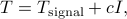
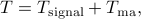
A possible generalization of this idea is to allow the noise component to have a moving-average (MA) spectrum [1] . Thus, we decompose as
.
A possible generalization of this idea is to allow the noise component to have a moving-average (MA) spectrum [1] . Thus, we decompose as
where  is a covariance matrix corresponding to a MA process. Let
  be a companion matrix of size
  and
and
![begin{array}{rl} B:=&[1,; 0,; ldots,; 0]^prime, C:=&[c(1),;c(2), ldots, c(m)]. end{array}](eqs/695089749-130.png)
Then
![T_{rm{ma}}=left[ begin{array}{ccccc} c(0) & ldots & c(m) & 0& ldots vdots & ddots & & ddots &ddots c(m)^* & ddots& & & 0 & ddots & & & vdots &ddots & & & end{array} right],](eqs/1030951066-130.png)
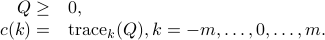
is the covariance matrix of a MA process if and only if there exist a  such that
![left[ begin{array}{cc} P-A^*PA & C^*-A^*PB C-B^*PA & c(0)-B^*PB end{array} right]geq0. hspace*{3cm} (a)](eqs/46214377-130.png)
This is a consequence of the KYP positive-real lemma [1]. Assuming that  is the order of the MA process, it is natural to subtract the maximum amount of noise from . Thus we are called to solve

This decomposition is obtained using routine MA_decomp.m which in turn uses the convex optimization package cvx.
An alternative approach is proposed in [2].
Let ![[q(0), ldots, q(m)]](eqs/1450623641-130.png) be the vector of the coefficients of a th order MA filter, and let
be the vector of the coefficients of a th order MA filter, and let

be the corresponding covariance sequence of the output of the filter driven by white noise with unit variance. Then
![c(k)= {rm trace}_kleft(left[ begin{array}{c} q(0) vdots q(m) end{array} right][q(0)^*, ldots, q(m)^*] right), ~k=-m, ldots, 0,ldots, m,](eqs/1221467401-130.png)
where  denotes the sum of the
  th sub-diagonal of a matrix.
This was relaxed to the constraint used in [2] as follows
th sub-diagonal of a matrix.
This was relaxed to the constraint used in [2] as follows
Example
Consider the following sequence

with  and
and  ,
,  , and the noise component
  generated by a MA filter driven by
white noise (complex with independent real and imaginary parts). The MA filter is
generated by a MA filter driven by
white noise (complex with independent real and imaginary parts). The MA filter is  rd with zeros at
  ,
,  , and
, and  respectively.
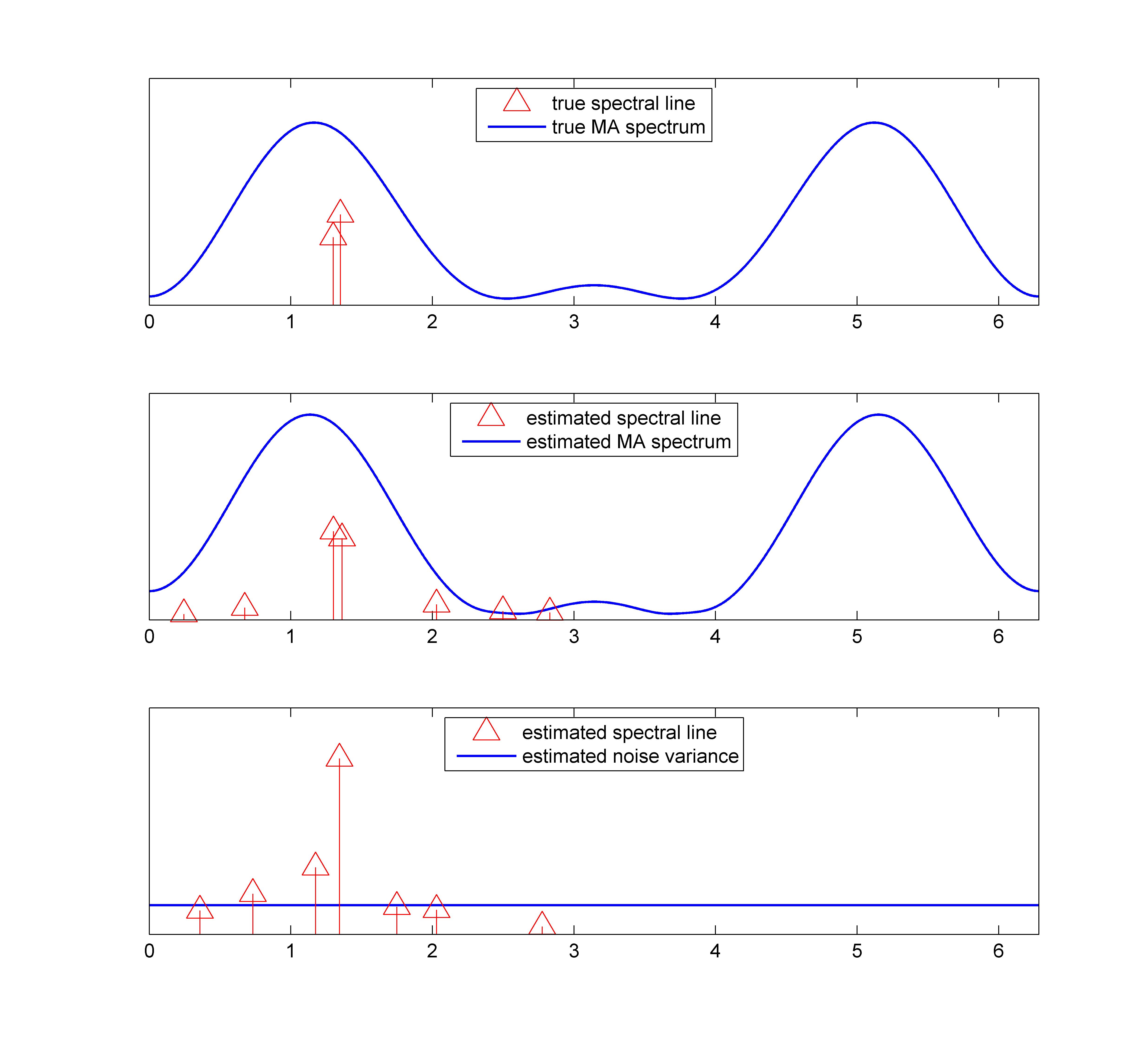
The first figure below shows the true spectral lines marked with arrows superimposed on the MA spectrum. The figure in the middle shows the estimated spectral lines and the estimated rd order MA spectrum. There are two dominant spectral lines locate very closely
to the true values. The figure at the bottom shows the estimate when the noise component is taken to be white.
The blue line shows the noise variance. In this case, only one dominant spectral line is detected near the true ones.
 |
Reference
[1] T.T. Georgiou, “Decomposition of Toeplitz matrices via convex optimization,” IEEE Signal Processing Letters, 13(9): 537-540, September 2006.
[2] P. Stoica, L. Du, J. Li and T. Georgiou, “A new method for moving-average parameter estimation”, Signals, Systems and Computers (ASILOMAR), 2010 Conference Record of the Forty Fourth Asilomar Conference on, 1817–1820, 2010.