% System parameters:
omval = logspace(5,7,300);  % temporal frequencies

% beam parameters
alpha = 5e-8; mu = 1.88e-7; ell = 240e-6; EI = 7.55e-12;

% convenience variables
a4 = EI/(ell^4); a3 = EI/(ell^3);

dom = domain(0,1);  % domain, y \in [0, 1]
y = chebfun('y',dom);
D1 = diff(dom,1); % first-order differentiation operator

% fone(y) = 1; fzero(y) = 0;
fone = chebfun(1,dom); fzero = chebfun(0,dom);

% Boundary conditions on the right end:
Wa = [1, 0, 0, 0; 0, 1, 0, 0; zeros(2,4)];
r = [0; 0; 0; (1/a3)]; % non-homogeneous boundary conditions

% Computing frequency responses
H1 = zeros(length(omval),1); KE = zeros(length(omval),1);
PE = zeros(length(omval),1);

for indom = 1:length(omval)

    om = omval(indom);

    % boundary conditions on the left end
    Wb = [zeros(2,4); ...
        0, 0, 1, 0; ...
        0, 0, 0, (1 + alpha*1i*om)];

    % system coefficients
    A0 = [-mu*om*om*fone, fzero, fzero, fzero, a4*(1 + alpha*1i*om)*fone];

    % solving integral boundary value problem
    % intbvp solves a scalar boundary value problem using the integral
    % representation
    % (type 'help intbvp' for more information on how to use intbvp)
    % intbvp.m is included in the download zip-folder
    [f,fder] = intbvp(A0,fzero,Wa,Wb,r);

    % frequency responses
    % 1) with the output g(t) = phi(1,t) = f(1,t)
    H1(indom) = f(1);

    % 2) with the output f(y,t) = phi(y,t)
    % kinetic energy: KE = 0.5*integrate_{0}^{1} (f??(y))^2 dy
    KE(indom) = 0.5*norm(D1*D1*f)^2;

    % potential energy: PE = 0.5*om*om*integrate_{0}^{1} f(y)^2 dy
    PE(indom) = 0.5*norm(om*f)^2;

end

% total energy: TE = PE + KE
TE = KE + PE;
Boundary actuation: an Euler-Bernoulli beam
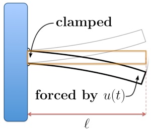 |
The vertical displacement of an Euler-Bernoulli beam that is clamped at the left end and subject to a boundary actuation at the other end is governed by
![begin{array}{rcl} mu , phi_{tt} (y, t) , + , {displaystyle frac{alpha , E_{I}}{ell^{4}}} , phi_{tyyyy}(y,t) , + , {displaystyle frac{E_{I}}{ell^{4}}} , phi_{yyyy}(y,t) & !! = !! & 0, ;; y in left[ , 0, 1 , right] [0.5cm] phi(0, t) ; = ; phi_{y}(0, t) & !! = !! & 0 [0.4cm] phi_{yy}( 1, t ) ; = ; 0, ;;; {displaystyle frac{alpha , E_{I}}{ell^{3}}} , phi_{tyyy}(1, t) , + , {displaystyle frac{E_{I}}{ell^{3}}} , phi_{yyy}(1, t) & !! = !! & u(t) end{array}](eqs/6526122142977153027-130.png)
where
 | — | vertical displacement of the beam |
 | — | force acting on the tip |
 | — | length of the beam |
 | — | mass per unit length of the beam |
 | — | flexural stiffness |
 | — | Voigt damping factor. |
The outputs are given by
![begin{array}{rcl} g (t) & !! = !! & phi(1,t) [0.15cm] f (y, t) & !! = !! & phi(y, t). end{array}](eqs/2673647037006230887-130.png)
Application of the temporal Fourier transform yields
![begin{array}{rcl} left( {displaystyle frac{E_{I}}{ell^{4}} left( 1 , + , mathrm{i} , omega , alpha right) D^{(4)} , - , omega^2 , mu } right) , phi (y, omega) & !! = !! & 0 [0.45cm] phi(0, omega) ; = ; D^{(1)} , phi(0, omega) & !! = !! & 0 [0.25cm] D^{(2)} , phi( 1, omega) ; = ; 0, ;;; {displaystyle frac{E_{I}}{ell^{3}} left( 1 , + , mathrm{i} , omega , alpha right) } , D^{(3)} , phi(1, omega) & !! = !! & u(omega). end{array}](eqs/3619645815926670013-130.png)
Matlab codes
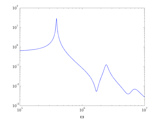
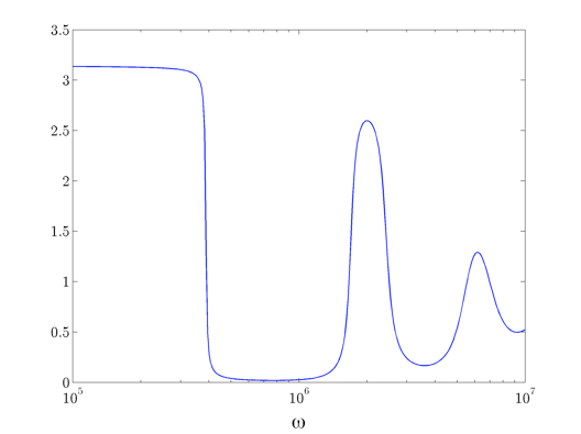
Plot the magnitude and phase of the transfer function from  to
to  .
.
loglog(omval,abs(H1),'b-','LineWidth',1.1)
xlab = xlabel('\omega', 'interpreter', 'tex');
set(xlab, 'FontName', 'cmmi10', 'FontSize', 20);
h = get(gcf,'CurrentAxes');
set(h, 'FontName', 'cmr10', 'FontSize', 15);

semilogx(omval,unwrap(angle(H1)),'b-','LineWidth',1.1)
xlab = xlabel('\omega', 'interpreter', 'tex');
set(xlab, 'FontName', 'cmmi10', 'FontSize', 20);
h = get(gcf,'CurrentAxes');
set(h, 'FontName', 'cmr10', 'FontSize', 15);
 |
 |
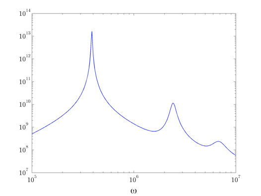
Plot the total energy of the beam arising from boundary actuation.
loglog(omval,TE,'b-','LineWidth',1.1)
xlab = xlabel('\omega', 'interpreter', 'tex');
set(xlab, 'FontName', 'cmmi10', 'FontSize', 20);
h = get(gcf,'CurrentAxes');
set(h, 'FontName', 'cmr10', 'FontSize', 15);
 |