|
One-dimensional heat equation
Let a one-dimensional heat equation with homogenous Dirichlet boundary
conditions and zero initial conditions be subject to spatially and temporally
distributed forcing
![begin{array}{rcl} phi_{t}(y,t) & !! = !! & phi_{yy}(y,t) , + , d(y,t), ;;; y in left[ -1, 1 right] [0.15cm] phi(pm 1, t) & !! = !! & 0, ;;; phi(y,0) ; = ; 0. end{array}](eqs/6077491061876695712-130.png)
The second derivative operator with Dirichlet boundary conditions is
self-adjoint with a complete set of orthonormal eigenfunctions,  , ,  . This information can
be used to diagonalize operator . This information can
be used to diagonalize operator  which facilitates
straightforward determination of the frequency response. For systems with
spatially varying coefficients and non-normal generators the frequency
response analysis is typically done numerically using finite dimensional
approximations of the differential operators. For example, the pseudospectral
method with which facilitates
straightforward determination of the frequency response. For systems with
spatially varying coefficients and non-normal generators the frequency
response analysis is typically done numerically using finite dimensional
approximations of the differential operators. For example, the pseudospectral
method with  collocation points can be used to transform
the frequency response operator into an collocation points can be used to transform
the frequency response operator into an  matrix. However, for systems
with differential operators of high order, spectral differentiation matrices
may be poorly conditioned and implementation of boundary conditions may be
challenging. In our method, numerical approximation of differential operators
in the evolution equation is avoided by first recasting the system into
corresponding two point boundary value problems and then using
state-of-the-art techniques for solving the resulting boundary value problems
with accuracy comparable to machine precision. matrix. However, for systems
with differential operators of high order, spectral differentiation matrices
may be poorly conditioned and implementation of boundary conditions may be
challenging. In our method, numerical approximation of differential operators
in the evolution equation is avoided by first recasting the system into
corresponding two point boundary value problems and then using
state-of-the-art techniques for solving the resulting boundary value problems
with accuracy comparable to machine precision.
Two point boundary value representations of  , ,  , and , and

Application of the temporal Fourier transform yields the two point
boundary value representation of the frequency response operator
,
where
 | — | imaginary unit |
 | — | temporal frequency |
| | — | second-order differential operator in  |
 | — | point evaluation functional at the boundary  . . |
|
|
The two point boundary value representation for the adjoint of the frequency response operator,
, is given by
The representation of the operator is obtained by combining
the two point boundary value representations of and .
As illustrated in Fig.  , this can be achieved by setting , this can be achieved by setting  in in  , ,
Note that svdfr.m utilizes the integral form of a two point boundary value representation of
. This procedure yields accurate results even for
systems with high order differential operators and poorly-scaled coefficients.
Integral form of a differential equation
We next illustrate the procedure for converting the differential equation
into its corresponding integral form. By
introducing an auxiliary variable
and by integrating  we obtain we obtain
Here,  and and  denote the indefinite integration operators of degrees one and two,
the vector denote the indefinite integration operators of degrees one and two,
the vector
![mathbf{k} = left[ begin{array}{cc} k_{2} & k_{1} end{array} right]^T](eqs/2435033097924618306-130.png) contains the constants of integration which are to be determined from the boundary conditions, and
contains the constants of integration which are to be determined from the boundary conditions, and
The integral form of the 1D heat equation is obtained by substituting  into , into ,
Now, by observing that
we can use  to express the constants of integration to express the constants of integration  in terms of in terms of  , ,
Finally, substitution of  into into  yields an equation for , yields an equation for ,
This equation only contains indefinite integration operators and point evaluation functionals which
are known to be well-conditioned.
Matlab codes
om = 0;
dom = domain(-1,1);
y = chebfun('y',dom);
fone = chebfun(1,dom);
fzero = chebfun(0,dom);
A0{1} = [-1i*om*fone, fzero, fone];
B0{1} = -fone;
C0{1} = fone;
Wa0{1} = [1, 0];
Wb0{1} = [1, 0];
Nsigs = 25;
LRfuns = 1;
[Sfun, Sval] = svdfr(A0,B0,C0,Wa0,Wb0,LRfuns,Nsigs);
Sa = (4./(([1:Nsigs].*pi).^2)).';
Sf1 = sin((1/sqrt(Sa(1))).*(y+1));
Sf2 = sin((1/sqrt(Sa(2))).*(y+1));
norm(Sval - Sa)
ans =

   5.4288e-15
Singular values of the frequency response operator: svdfr versus analytical results.
plot(1:Nsigs,Sval,'bx','LineWidth',1.25,'MarkerSize',10)
hold on
plot(1:Nsigs,Sa,'ro','LineWidth',1.25,'MarkerSize',10);
xlab = xlabel('n', 'interpreter', 'tex');
set(xlab, 'FontName', 'cmmi10', 'FontSize', 20);
h = get(gcf,'CurrentAxes');
set(h, 'FontName', 'cmr10', 'FontSize', 20, 'xscale', 'lin', 'yscale', 'lin');
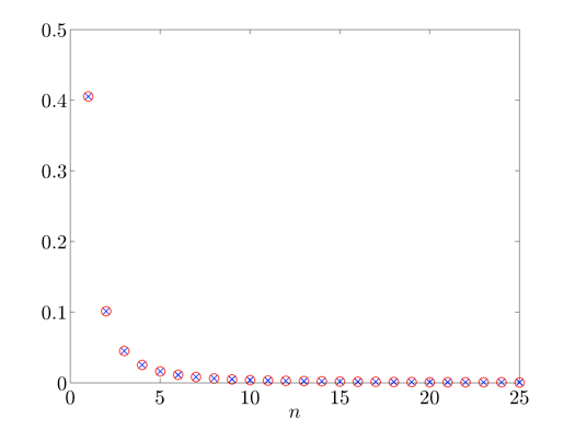 |
Twenty five largest singular values of the frequency response operator.
|
The principal singular function: svdfr versus analytical results.
hold off; plot(y,-Sfun(:,1),'bx-','LineWidth',1.25,'MarkerSize',10)
hold on; plot(y,Sf1,'ro-','LineWidth',1.25,'MarkerSize',10);
xlab = xlabel('y', 'interpreter', 'tex');
set(xlab, 'FontName', 'cmmi10', 'FontSize', 20);
h = get(gcf,'CurrentAxes');
set(h, 'FontName', 'cmr10', 'FontSize', 20, 'xscale', 'lin', 'yscale', 'lin');
axis tight
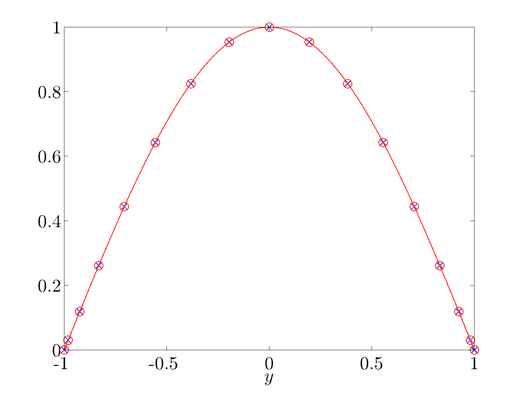 |
The principal singular function of the frequency response operator.
|
The singular function corresponding to the second largest singular value:
svdfr versus analytical results.
hold off; plot(y,Sfun(:,2),'bx-','LineWidth',1.25,'MarkerSize',10)
hold on; plot(y,Sf2,'ro-','LineWidth',1.25,'MarkerSize',10);
xlab = xlabel('y', 'interpreter', 'tex');
set(xlab, 'FontName', 'cmmi10', 'FontSize', 20);
h = get(gcf,'CurrentAxes');
set(h, 'FontName', 'cmr10', 'FontSize', 20, 'xscale', 'lin', 'yscale', 'lin');
axis tight
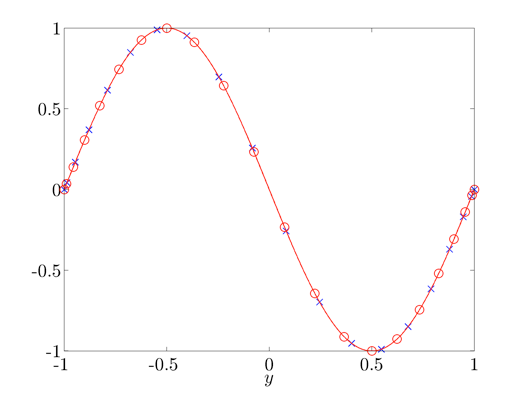 |
The singular function of the frequency response operator corresponding to the second largest
singular value.
|
|
![begin{array}{rcl} left( D^{(2)} , - , mathrm{i} , omega right) phi(y) & !! = !! & -d(y) [0.15cm] left( left[ begin{array}{c} 1 [0.1cm] 0 end{array} right] E_{-1} , + , left[ begin{array}{c} 0 [0.1cm] 1 end{array} right] E_{+1} right) phi(y) & !! = !! & left[ begin{array}{c} 0 [0.1cm] 0 end{array} right] end{array} hspace{3.0cm} mathrm{(1)}](eqs/3002208525606426121-130.png)
![begin{array}{rcl} left( D^{(2)} , + , mathrm{i} , omega right) psi(y) & !! = !! & f(y) [0.15cm] g(y) & !! = !! & -psi(y) [0.15cm] left( left[ begin{array}{c} 1 [0.1cm] 0 end{array} right] E_{-1} , + , left[ begin{array}{c} 0 [0.1cm] 1 end{array} right] E_{+1} right) psi(y) & !! = !! & left[ begin{array}{c} 0 [0.1cm] 0 end{array} right]. end{array}](eqs/433950289553441871-130.png)
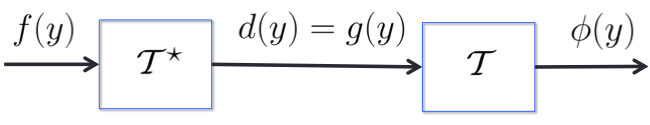
![mathcal{T} mathcal{T}^{star}!!: ~ left{ begin{array}{rcl} left[ begin{array}{cc} left( D^{(2)} , - , mathrm{i} , omega right) & -I [0.15cm] 0 & left( D^{(2)} , + , mathrm{i} , omega right) end{array} right] left[ begin{array}{c} phi(y) [0.15cm] psi(y) end{array} right] & !! = !! & left[ begin{array}{c} 0 [0.15cm] I end{array} right] f(y) [0.5cm] phi (y) & !! = !! & left[ begin{array}{cc} I & 0 end{array} right] left[ begin{array}{c} phi (y) [0.1cm] psi (y) end{array} right] [0.5cm] left( left[ begin{array}{c} 1 [0.1cm] 0 end{array} right] E_{-1} , + , left[ begin{array}{c} 0 [0.1cm] 1 end{array} right] E_{+1} right) phi(y) & !! = !! & left[ begin{array}{c} 0 [0.1cm] 0 end{array} right] [0.6cm] left( left[ begin{array}{c} 1 [0.1cm] 0 end{array} right] E_{-1} , + , left[ begin{array}{c} 0 [0.1cm] 1 end{array} right] E_{+1} right) psi(y) & !! = !! & left[ begin{array}{c} 0 [0.1cm] 0 end{array} right]. end{array} right.](eqs/8086892661573860403-130.png)
![nu(y) ; = ; left[ D^{(2)} , phi right] (y) ; =: ; phi'' (y) hspace{6.0cm} mathrm{(2)}](eqs/178937555630711437-130.png)
![begin{array}{rcl} phi'(y) & = & {displaystyle int_{-1}^{y} nu(eta_{1}) , mathrm{d} eta_{1}} ; + ; k_1 ~ = ~ left[ J^{(1)} , nu right] (y) ; + ; k_1 [0.35cm] phi(y) & = & {displaystyle int_{-1}^{y} left( int_{-1}^{eta_{2}} nu(eta_{1}) , mathrm{d} eta_{1} right) mathrm{d} eta_{2} ; + ; k_{1} left( y , + , 1 right) ; + ; k_{2}} [0.4cm] & = & left[ J^{(2)} , nu right] (y) ; + ; K^{(2)} , mathbf{k}. end{array} hspace{1.5cm} mathrm{(3)}](eqs/3915249027210281089-130.png)
![K^{(2)} ; = ; left[ begin{array}{cc} 1 & (y + 1) end{array} right].](eqs/6271119260619181692-130.png)
![begin{array}{rcll} left( I - mathrm{i} omega J^{(2)} right) nu(y) , - , mathrm{i} omega , K^{(2)} , mathbf{k} & !! = !! & - d(y) & hspace{0.5cm} mathrm{(4a)} [0.4cm] left[ begin{array}{cc} 1 & 0 1 & 2 end{array} right] left[ begin{array}{c} k_2 k_1 end{array} right] ; + ; left( left[ begin{array}{c} 1 0 end{array} right] E_{-1} , + , left[ begin{array}{c} 0 1 end{array} right] E_{+1} right) left[ J^{(2)} nu right] (y) & !! = !! & left[ begin{array}{c} 0 0 end{array} right]. & hspace{0.5cm} mathrm{(4a)} end{array}](eqs/3175655364539582889-130.png)
![E_{-1} left[ J^{(1)} nu right] (y) ; = ; {displaystyle int_{-1}^{-1} nu(eta) , mathrm{d} eta} ; = ; 0](eqs/5218163849500979667-130.png)
![begin{array}{rcl} left[ begin{array}{c} k_{2} [0.1cm] k_{1} end{array} right] & !! = !! & - {displaystyle frac{1}{2}} left[ begin{array}{rc} 2 & 0 [0.1cm] -1 & 1 end{array} right] left[ begin{array}{c} 0 [0.1cm] 1 end{array} right] E_{+1} , left[ J^{(2)} , nu right] (y) [0.5cm] & !! = !! & - {displaystyle frac{1}{2}} left[ begin{array}{c} 0 [0.1cm] 1 end{array} right] E_{+1} , left[ J^{(2)} , nu right] (y). hspace{5cm} mathrm{(5)} end{array}](eqs/6418866729015168359-130.png)