|
LQRSP – Sparsity-Promoting Linear Quadratic Regulator
Introduction
lqrsp.m is a Matlab function for the design of sparse and block
sparse state-feedback gains that minimize the variance amplification
(i.e., the  norm) of distributed systems. Our long-term
objective is to develop a toolbox for sparse feedback synthesis. This
will allow users to identify control configurations that strike a
balance between the performance and the sparsity of the controller and
to examine the influence of different control configurations on the
performance of distributed systems. norm) of distributed systems. Our long-term
objective is to develop a toolbox for sparse feedback synthesis. This
will allow users to identify control configurations that strike a
balance between the performance and the sparsity of the controller and
to examine the influence of different control configurations on the
performance of distributed systems.
The design procedure consists of two steps:
Identification of sparsity patterns by incorporating
sparsity-promoting penalty functions into the optimal control problem.
Optimization of feedback gains subject to structural constraints
determined by the identified sparsity patterns.
Problem formulation
Consider the following control problem
where  is the exogenous input signal and is the exogenous input signal and  is the performance output.
The matrix is the performance output.
The matrix  is a state feedback gain, is a state feedback gain,  and and  are the state and control performance weights, and the closed-loop system is given by
We study the sparsity-promoting optimal control problem
in which the closed-loop norm  is augmented by a function is augmented by a function  that
counts the number of nonzero elements in the feedback gain matrix . For example, that
counts the number of nonzero elements in the feedback gain matrix . For example,
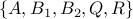
As the parameter  varies over varies over  , the solution traces the optimal
trade-off path between the quadratic performance and the feedback gain sparsity. , the solution traces the optimal
trade-off path between the quadratic performance and the feedback gain sparsity.
 |
Increased emphasis on sparsity encourages sparser control
architectures at the expense of deteriorating system's performance.
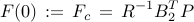
For  the optimal controller the optimal controller
is obtained from the positive definite solution of the algebraic Riccati equation
Control architectures for  depend on interconnections in
the distributed plant and the state and control performance weights. depend on interconnections in
the distributed plant and the state and control performance weights.
|
After a desired level of sparsity is achieved,
we fix the sparsity structure  and find the optimal structured feedback
gain . and find the optimal structured feedback
gain .
Relaxations of cardinality function
In addition to the cardinality function, we also consider several sparsity-promoting relaxations including
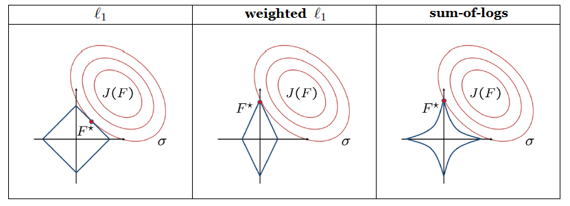
To illustrate the sparsity-promoting properties of these relaxations,
let us consider the problem of finding the sparsest feedback gain that
provides a given level of performance  . Convex ( . Convex ( and weighted norm) and non-convex (sum-of-logs) relaxations
of the cardinality function lead to
and weighted norm) and non-convex (sum-of-logs) relaxations
of the cardinality function lead to
The solution of the relaxed problem is the intersection of the constraint set  and the smallest sub-level set of
  that touches that touches  . .
Alternating direction method of multipliers (ADMM)
ADMM is a simple but powerful algorithm well-suited to large optimization problems. It blends the
separability of the dual decomposition with the superior convergence of the method of multipliers.
In the sparsity-promoting linear quadratic regulator problem, we use ADMM as the general purpose algorithm that
identifies sparsity patterns
provides good initial condition for structured design.
The algorithm consists of four steps:
Sketch of the algorithm
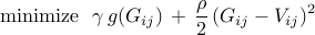
Solution to the G-minimization problem
Since all of the above mentioned sparsity-promoting penalty functions can be written as a
summation of componentwise functions, we can decompose the  -minimization problem into
sub-problems expressed in terms of the individual elements of , -minimization problem into
sub-problems expressed in terms of the individual elements of ,
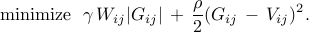
where
 This separability of the -minimization problem facilitates development of element-wise analytical
solutions.
This separability of the -minimization problem facilitates development of element-wise analytical
solutions.
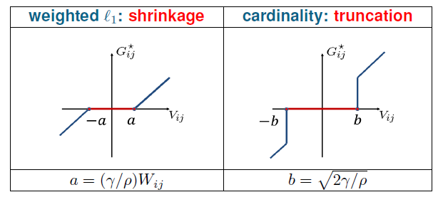
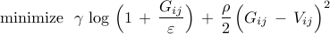
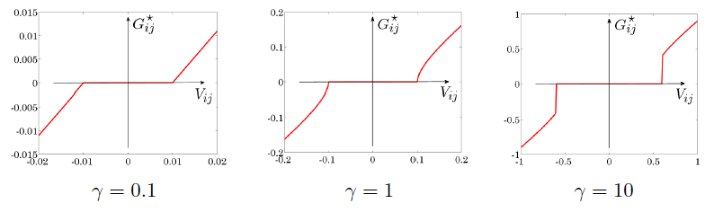
For sum-of-logs function, the solution to the -minimization sub-problem
depends on the parameters  , ,  , ,  . For example,
the solution of . For example,
the solution of
with  , ,  resembles the shrinkage operator for
small values of (e.g., resembles the shrinkage operator for
small values of (e.g.,  ), and it resembles the truncation operator
for large values of (e.g., ), and it resembles the truncation operator
for large values of (e.g.,  ). ).
Solution to the F-minimization problem
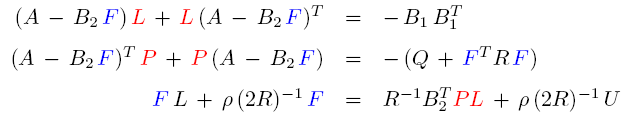
The necessary conditions for the optimality of the -minimization problem are given by
the three coupled nonlinear equations in the unknowns matrices ,  , and , and  , ,
For a fixed , the first two equations are Lyapunov equations for the closed-loop controllability
and observability gramians and , respectively; for fixed and , the third equation is
a Sylvester equation for . This structure of the necessary conditions for the optimality motivates
the following iterative scheme
We have shown that the difference between the feedback gains in two consecutive steps provides a
descent direction. This observation in conjunction with standard line search has allowed us
to establish convergence of the iterative scheme.
Polishing
The necessary conditions for the optimality of the structured linear quadratic regulator
problem are given by
where  denotes the entry-wise multiplication of two matrices, and denotes the entry-wise multiplication of two matrices, and  is the
structural identity. For example, is the
structural identity. For example,
We have used Newton's method and employed the conjugate gradient scheme to compute the Newton
direction efficiently.
Extension: Block sparsity
In many problems it is of interest to design feedback gains that have block sparse structure.
In view of this, we have also considered the optimal control problem that promotes sparsity
of the feedback gain at the level of the submatrices instead of at the level of the individual
elements.
The function that counts the number of nonzero submatrices is given by
where  and and  is the Frobenius norm.
We have also examined the following relaxations is the Frobenius norm.
We have also examined the following relaxations
 |
An example of a block sparse feedback gain with
submatrices of size 
Additional information is provided in the block sparsity example.
|
Description of lqrsp.m
Matlab Syntax
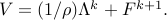
>> solpath = lqrsp(A,B1,B2,Q,R,options);
Our Matlab function lqrsp.m takes the matrices
and the input options and returns the -parameterized family of solutions to both the
sparsity-promoting optimal control problem (SP) and the structured problem (SH2).
Input options allows users to specify the following parameters
sparsity-promoting penalty function:  , ,  ,
or one of the relaxations ,
or one of the relaxations  with with  ; ;
values of and ;
maximum number of ADMM iterations;
maximum number of re-weighted iterations (if weighted or weighted sum of
Frobenius norms is used);
block size ![[n_i, , m_j]](eqs/6053709491426191049-130.png) of the submatrix
(if block sparsity is desired). of the submatrix
(if block sparsity is desired).
The -parameterized output solpath is a structure that contains
solpath.F – feedback gains resulting from the control problem (SP);
solpath.Fopt – feedback gains resulting from the structured control problem (SH2);
solpath.J – quadratic performance of the solutions to (SP);
solpath.Jopt – optimal quadratic performance of the solutions to (SH2);
solpath.nnz – number of nonzero elements (blocks) of optimal sparse (block sparse)
feedback gains;
solpath.gam – values of sparsity-promoting parameter .
help lqrsp
  Sparsity-Promoting Linear Quadratic Regulator

  Written by Fu Lin, January 2012

  Description:

  The sparsity-promoting linear quadratic regulator problem is solved using
  the alternating direction method of multipliers (ADMM)

        minimize J(F) + gamma * g(F)             (SP)

  where J is the closed-loop H2 norm, g is a sparsity-promoting penalty
  function, and gamma is the parameter that emphasizes the importance of
  sparsity.

  After the sparsity pattern has been identified, the structured H2 problem
  is solved

        minimize    J(F)
                                                                 (SH2)
        subject to  F belongs to identified sparsity pattern

  Syntax:

  solpath = lqrsp(A,B1,B2,Q,R,options)

  Inputs:

  (I)  State-space representation matrices {A,B1,B2,Q,R};

  (II) Options

      a) options.method specifies the sparsity-promoting penalty function g

         options.method = 'card'     --> cardinality function,
                        = 'l1'       --> l1 norm,
                        = 'wl1'      --> weighted l1 norm,
                        = 'slog'     --> sum-of-logs function,
                        = 'blkcard'  --> block cardinality function,
                        = 'blkl1'    --> sum of Frobenius norms,
                        = 'blkwl1'   --> weighted sum of Frobenius norms,
                        = 'blkslog'  --> block sum-of-logs function;

      b) options.gamval         --> range of gamma values;
      c) options.rho            --> augmented Lagrangian parameter;
      d) options.maxiter        --> maximum number of ADMM iterations;
      e) options.blksize        --> size of block sub-matrices of F;
      f) options.reweightedIter --> number of iterations for the reweighted
                                    update scheme.

  The default values of these fields are

  options.method         = 'wl1';
  options.gamval         = logspace(-4,1,50);
  options.rho            = 100;
  options.maxiter        = 1000;
  options.blksize        = [1 1];
  options.reweightedIter = 3.

  Output:

  solpath -- the solution path parameterized by gamma -- is a structure
  that contains:

  (1) solpath.F    --> feedback gains resulting from the control problem
                       (SP);
  (2) solpath.Fopt --> feedback gains resulting from the structured control
                       problem (SH2);
  (3) solpath.J    --> quadratic performance of the solutions to (SP);
  (4) solpath.Jopt --> optimal quadratic performance of the solutions to
                       (SH2);
  (5) solpath.nnz  --> number of nonzero elements (blocks) of optimal
                       sparse (block sparse) feedback gains;
  (6) solpath.gam  --> values of sparsity-promoting parameter gamma.

  Reference:

  F. Lin, M. Fardad, and M. R. Jovanovic
  ``Design of optimal sparse feedback gains via the alternating direction method of multipliers''
  IEEE Trans. Automat. Control, vol. 58, no. 9, pp. 2426-2431, September 2013.

  Additional information:

  http://www.umn.edu/~mihailo/software/lqrsp/
Acknowledgements
We would like to thank Stephen Boyd for encouraging us to develop
this software.
This project is supported in part by the National Science Foundation under
|
![begin{array}{rrcl} {bf state~equation}!!: & dot{x} & = & A , x ,+, B_1 , d ,+, B_2 , u [0.25cm] {bf performance~output}!!: & z & = & left[ begin{array}{c} Q^{1/2} 0 end{array} right] , x , + , left[ begin{array}{c} 0 R^{1/2} end{array} right] , u [0.5cm] {bf control~input}!!: & u & = & - , F , x end{array}](eqs/2141256092079558995-130.png)
![begin{array}{rcl} dot{x} & = & (A ,-, B_2 F) , x ,+, B_1 , d [0.25cm] z & = & left[ begin{array}{c} Q^{1/2} -,R^{1/2} F end{array} right] x. end{array}](eqs/7076251126697554418-130.png)

![F ;=; left[ begin{array}{cccc} 5 & 0 & 0 & 0 0 & 3.2 & 1.6 & 0 0 & -4 & 0 & 1 end{array} right] ~~~ Rightarrow ~~~ {rm{bf card}} , (F) ;=; 5.](eqs/3179681224735722348-130.png)
![begin{array}{c} {bf parameterized~family~of~feedback~gains}!!: [0.15cm] F (gamma) ~ := ~ {rm arg , min}_F left{ J(F) ; + ; gamma , {rm{bf card}} , (F) right} end{array}](eqs/661018926884376894-130.png)

![{bf structured}~{cal H}_2~{bf problem}!!: ~~ left{ begin{array}{ll} {rm minimize} & J(F) [0.2cm] {rm subject~to} & F in {cal S} end{array} right. hspace{5cm} {rm (SH2)}](eqs/6678614315974611017-130.png)
![begin{array}{rrcl} ell_1~{bf norm}!!: & g_1(F) & !! = !! & {displaystyle sum_{i, , j}} , | F_{ij} | [0.5cm] {bf weighted}~ell_1~{bf norm}!!: & g_2(F) & !! = !! & {displaystyle sum_{i, , j}} , W_{ij} | F_{ij} | [0.5cm] {bf sum}{rm-}{bf of}{rm-}{bf logs}!!: & g_3(F) & !! = !! & {displaystyle sum_{i, , j}} , log left( 1 , + , {displaystyle frac{| F_{ij} |}{varepsilon} } right), ~~ 0 , < , varepsilon , ll , 1. end{array}](eqs/2435952235945654338-130.png)
![begin{array}{ccc} begin{array}{c} {bf original~problem!!:} [0.25cm] begin{array}{ll} {rm minimize} & {rm{bf card}} , (F) [0.35cm] {rm subject~to} & J(F) , leq , sigma end{array} end{array} &~~ begin{array}{c} Rightarrow end{array} ~~& begin{array}{c} {bf relaxation!!:} [0.25cm] begin{array}{ll} {rm minimize} & g(F) [0.35cm] {rm subject~to} & J(F) , leq , sigma end{array} end{array} end{array}](eqs/4404536581742808930-130.png)
![begin{array}{ll} {rm minimize} & J(F) ; + ; gamma , g (G) [0.25cm] {rm subject~to} & F ; - ; G ; = ; 0 end{array}](eqs/5329615988508255447-130.png)

![begin{array}{rllll} bf{F !! - !! minimization~problem:} && F^{k+1} & !! := !! & {displaystyle {rm arg , min}_{F}} ; {cal L}_rho (F,G^k,Lambda^k) [0.35cm] bf{G !! - !! minimization~problem:} && G^{k+1} & !! := !! & {displaystyle {rm arg , min}_{G}} ; {cal L}_rho (F^{k+1},G,Lambda^k) [0.35cm] bf{Lambda !! - !! update~step:} && Lambda^{k+1} & !! := !! & Lambda^{k} ;+; rho left( F^{k+1} ; - ; G^{k+1} right) end{array}](eqs/7559214060659643287-130.png)
![{bf structured}~{cal H}_2~{bf problem}!!: ~~ left{ begin{array}{ll} {rm minimize} & J(F) [0.2cm] {rm subject~to} & F in {cal S} end{array} right.](eqs/4458905421536668354-130.png)


![begin{array}{rcl} (A , - , B_2 , F )^T P ~ + ~ P , (A , - , B_2 , F ) & = & - left( Q ,+, F^T R , F right) [0.25cm] (A , - , B_2 , F ) , L ,+, L , (A , - , B_2 , F )^T & = & -B_1 B_1^T [0.25cm] left[ left( R , F , - , B_2^T P right) L right] circ I_{cal S} & = & 0, end{array}](eqs/4736974792619070485-130.png)
![begin{array}{rcccl} F ; = ; left[ begin{array}{cccc} * & * & & {*} & * & * & & * & * & * & & * & * end{array} right] & & Rightarrow & & I_{cal S} ; = ; left[ begin{array}{cccc} 1 & 1 & & 1 & 1 & 1 & & 1 & 1 & 1 & & 1 & 1 end{array} right]. end{array}](eqs/5585993184713182779-130.png)
![begin{array}{rrcl} {bf sum~of~Frobenius~norms}!!: & g_4(F) & !! = !! & {displaystyle sum_{i, , j}} , | F_{ij} |_F [0.5cm] {bf weighted~sum~of~Frobenius~norms}!!: & g_5(F) & !! = !! & {displaystyle sum_{i, , j}} , W_{ij} | F_{ij} |_F [0.5cm] {bf generalized~sum}{rm!-!}{bf of}{rm!-!}{bf logs}!!: & g_6(F) & !! = !! & {displaystyle sum_{i, , j}} , log left( 1 , + , {displaystyle frac{| F_{ij} |_F}{varepsilon} } right), ~~ 0 , < , varepsilon , ll , 1. end{array}](eqs/8334597287522862916-130.png)