 systems coupled through the following dynamics
![[, cdot ,]_{ij}](eqs/8267110984842165856-130.png) denotes the
denotes the  th block of a matrix and
 and
and  are set to identity matrices.
  control input and
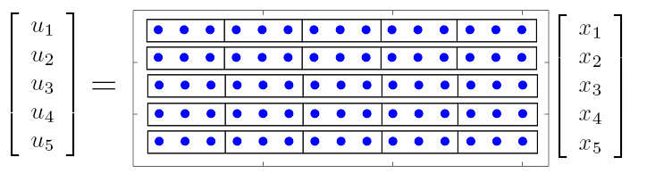
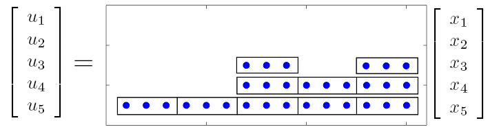
  states, the feedback gain matrix can be partitioned
into
states, the feedback gain matrix can be partitioned
into  submatrices as illustrated in the figure. We are interested in obtaining feedback
gains with small number of block submatrices.
submatrices as illustrated in the figure. We are interested in obtaining feedback
gains with small number of block submatrices. % Block sparsity example % number of systems N = 5; % size of each system nn = 3; mm = 1; % use cyclic condition to obtain unstable system a = ones(1,nn); b = 1.5*(sec(pi/nn))*a; % state-space representation of each system Aa = -diag(a) + diag(b(2:nn),-1); Aa(1,nn) = -b(1); Bb1 = diag(b); Bb2 = zeros(nn,1); Bb2(1) = b(1); % non-symmetric weighted Laplacian matrix % adjacency matrix Ad = toeplitz([1 0 0 1 0 0 1 0 0 1 0 0 1 0 0]); for i = 1 : N for j = 1 : N if i ~= j cij = 0.5 * ( i - j ); else cij = 0; end Ad( nn*(i-1)+1 : nn*i, nn*(j-1)+1 : nn*j) = cij * eye(nn); end end % take the sum of each row d = sum(Ad,2); % form the Laplacian matrix L = Ad - diag(d); % state-space representation of the interconnected system A = kron(eye(N), Aa) - L; B1 = kron(eye(N), Bb1); B2 = kron(eye(N), Bb2); Q = eye(nn*N); R = eye(N); % compute block sparse feedback gains options_blkwl1 = struct('method','blkwl1','gamval', ... logspace(-1,log10(5),50),'rho',100,'maxiter',1000,'blksize',[1 3], ... 'reweightedIter',1); tic solpath_blkwl1 = lqrsp(A,B1,B2,Q,R,options_blkwl1); toc % compute element sparse feedback gains options_wl1 = struct('method','wl1','gamval', ... logspace(-1,log10(5),50),'rho',100,'maxiter',1000,'blksize',[1 1], ... 'reweightedIter',1); tic solpath_wl1 = lqrsp(A,B1,B2,Q,R,options_wl1); toc
Block sparsity: An example from bio-chemical reaction
 |
Consider a network of ![dot{x}_i , = , [A]_{ii} , x_i , - , frac{1}{2} sum_{ j ,=, 1 }^N (i - j) , (x_i , - , x_j) , + , [B_1]_{ii} , d_i ,+, [B_2]_{ii} , u_i,](eqs/8966637197022143107-130.png)
where ![[A]_{ii} , = , left[ begin{array}{rrr} -1 & 0 & -3 3 & -1 & 0 0 & 3 & -1 end{array} right], ~~ [B_1]_{ii} , = , left[ begin{array}{ccc} 3 & 0 & 0 0 & 3 & 0 0 & 0 & 3 end{array} right], ~~ [B_2]_{ii} , = , left[ begin{array}{c} 3 0 0 end{array} right].](eqs/2790440546242123113-130.png)
Each system models a cyclic interconnection that arises in bio-chemical reactions
(e.g., see Jovanovic et al. ’08).
The performance weights |
 |
Since each subsystem has |
In this example, we use the weighted sum of Frobenius norms to design optimal block sparse feedback
gains. To compare with elementwise sparsity, we also use the weighted  norm for optimal
sparse feedback design. In both cases, we set
norm for optimal
sparse feedback design. In both cases, we set  ,
,  and select
  logarithmically-spaced points for
 ![gamma in [0.1, , 5].](eqs/3246205059139060419-130.png)
We next show the Matlab code and the computational results obtained using lqrsp.m.
Matlab code
Computational results
Download Matlab code block_sparsity.m to reproduce these figures.
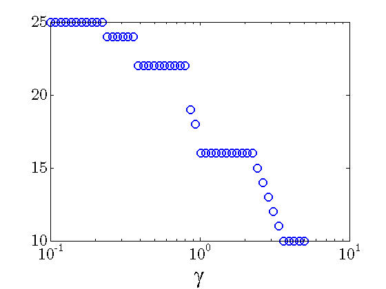 |
Number of nonzero block submatrices decreases with |
 .
.
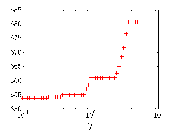 |
Quadratic performance deteriorates with |
The following example illustrates two feedback gains resulting from the block sparse and sparse feedback
designs. These feedback gains have close quadratic performance,
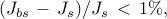 and the same number of nonzero elements, but different number of nonzero block submatrices.
Furthermore, as illustrated below, the optimal sparse feedback gain requires
and the same number of nonzero elements, but different number of nonzero block submatrices.
Furthermore, as illustrated below, the optimal sparse feedback gain requires  more communication
links than the optimal block sparse feedback gain.
more communication
links than the optimal block sparse feedback gain.
 |
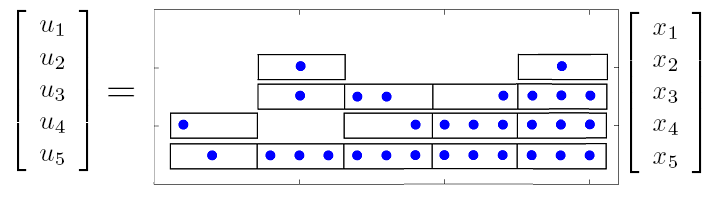
Structure of the optimal block sparse feedback gain. The algorithm with the weighted sum of
Frobenius norms and
|
 yields
  (black boxes) and
 (blue dots).
  do not need to be actuated.
 |
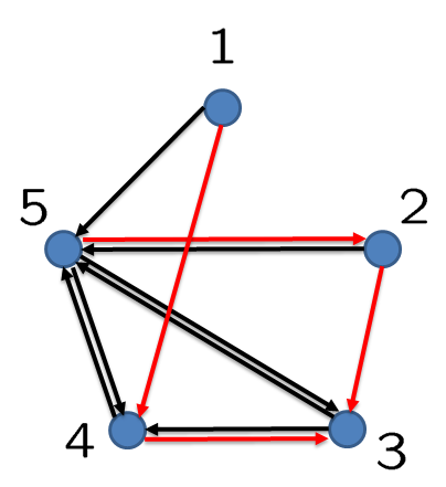
Structure of the optimal sparse feedback gain. The algorithm with the weighted |
 yields
 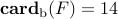 (black boxes) and
 |
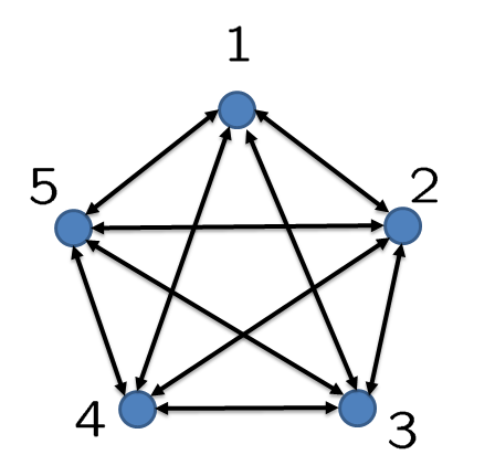
Communication graph of the optimal block sparse feedback gain. |
 |
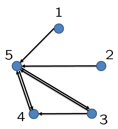
Communication graph of the optimal sparse feedback gain.
|