Performance evaluation
 |
We solve the problem |
 , where
  identifies the value
of the regularization parameter
identifies the value
of the regularization parameter  and
and Customized IP method vs CVX
Here, we compare the performance of our customized primal-dual
interior-point algorithms with CVX. The direct algorithm uses Cholesky
factorization to compute the search direction, and the indirect algorithm
uses the matrix-free preconditioned conjugate gradients method (with
diagonal preconditioner). We set  and choose the state weight that
penalizes the mean-square deviation from the network average
and choose the state weight that
penalizes the mean-square deviation from the network average  .
.
Figures below compare scalability of direct and indirect algorithms with CVX.
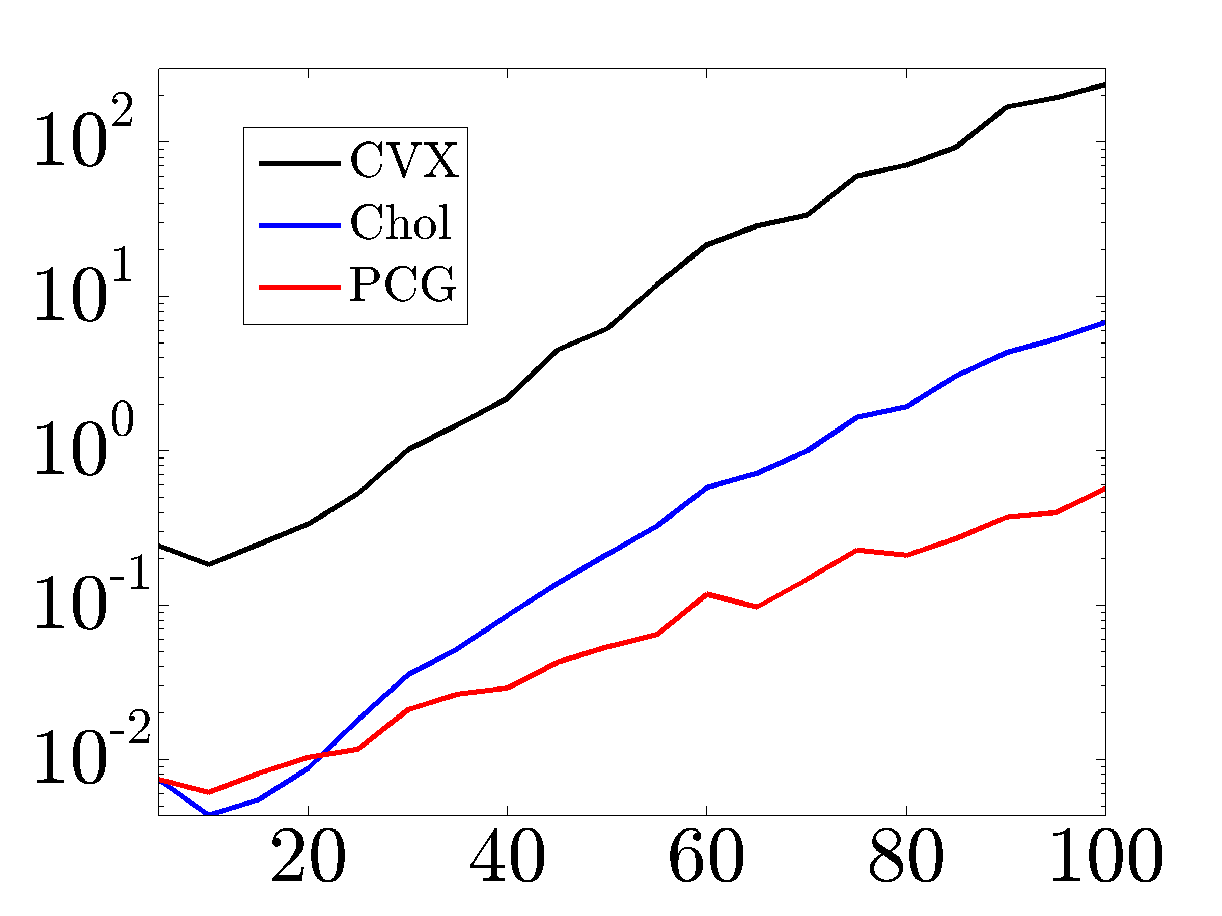 |
Solve times in seconds for networks with growing number of nodes. As the size of the network increases, implementations based on Cholesky factorization and PCG method significantly outperform CVX. |
 ,
,  , and
, and  vs
vs 
The solid lines in the following figures show ratios of the running times
for CVX and our customized algorithms versus the number of nodes. As
indicated by the dashed red lines, on average, algorithms based on Cholesky
factorization and PCG method are about  and
and  times faster than CVX
(for network sizes that can be handled by CVX).
times faster than CVX
(for network sizes that can be handled by CVX).
 |
|
 vs
vs
 |
|
 vs
vs Influence of the regularization parameter on performance
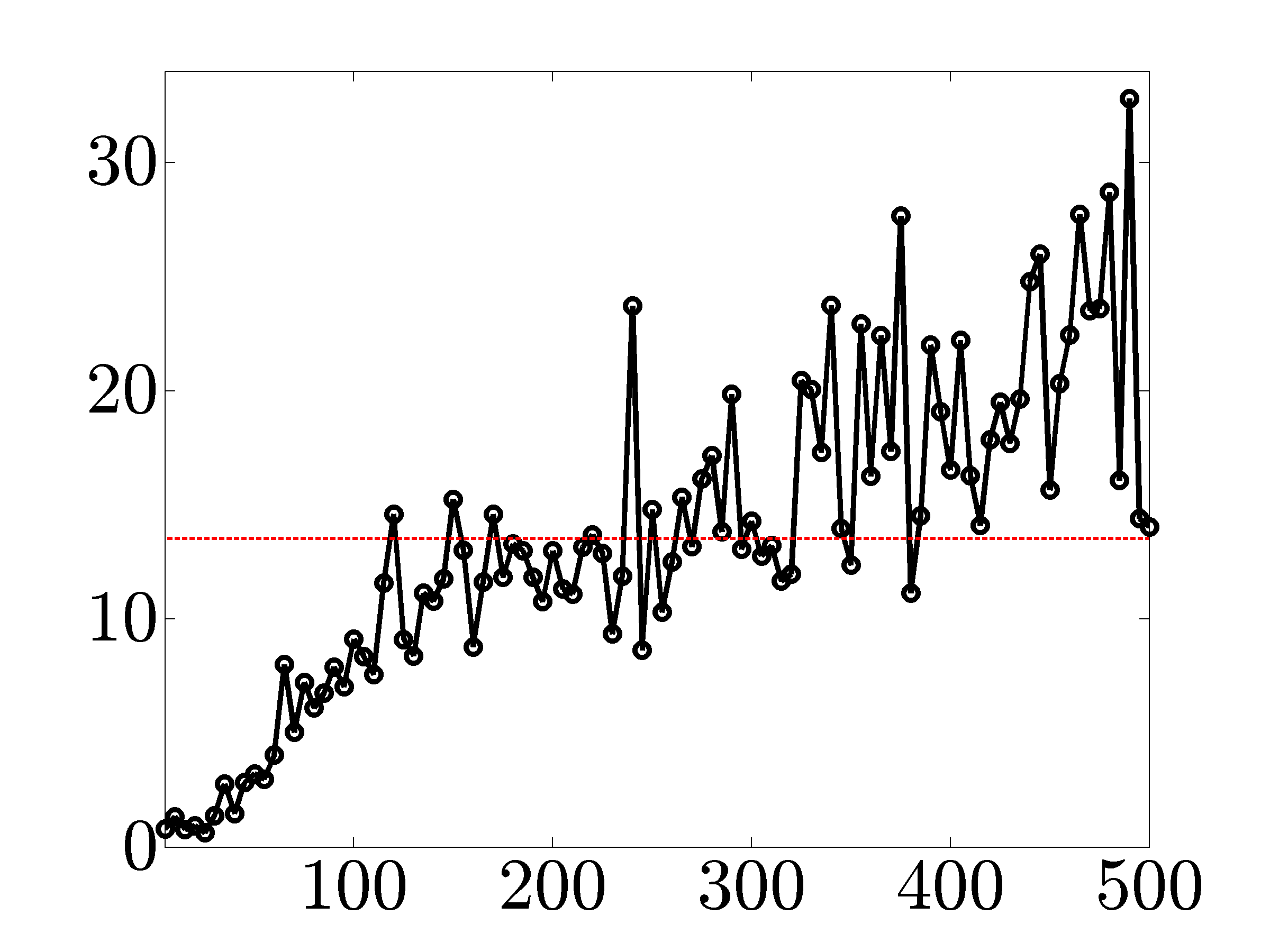
Next figure illustrates the influence of the regularization parameter
 on the performance of the matrix-free PCG algorithm for an
Erdos-Renyi network with
on the performance of the matrix-free PCG algorithm for an
Erdos-Renyi network with  nodes.
 |
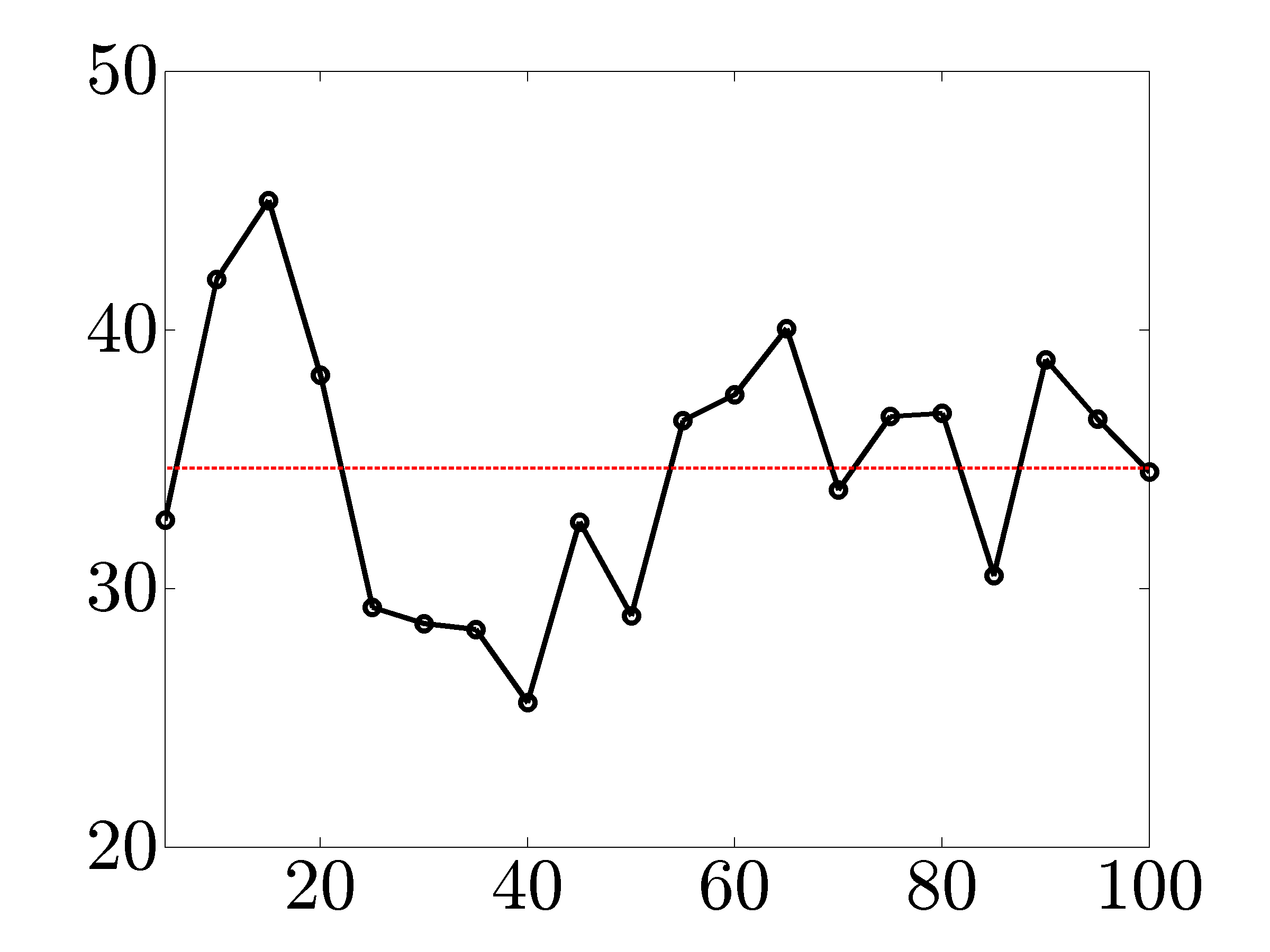
Duality gap vs cumulative number of PCG iterations. The total number of PCG iterations decreases with |
 for
for
 to
to  for
for  . Thus,
the indirect method computes sparser solutions more efficiently. Furthermore,
each PCG iteration takes about
. Thus,
the indirect method computes sparser solutions more efficiently. Furthermore,
each PCG iteration takes about  seconds. These results are consistent
with the observations made by
seconds. These results are consistent
with the observations made by
 -regularized logistic regression problems.
 IP method vs proximal algorithms
To compare the performance of proximal gradient and Newton methods and illustrate scalability of these algorithms, we solve the problem of growing Erdos-Renyi networks with different number of nodes.
Figures below compare scalability of primal-dual IP algorithm, proximal gradient (proxBB), and proximal Newton (proxN) algorithms.
 |
Solve times in seconds for networks with growing number of nodes. As the size of the network increases, both proximal gradient and proximal Newton algorithms significantly outperform the IP method. |
 ,
,  , and
, and  vs
vs The solid lines in the following figures show ratios of the solve times
between the IP method and the proximal algorithms versus the number of nodes. As
indicated by the dashed lines, on average, proximal gradient and proximal Newton
algorithms are about  and
and  times faster than the customized IP algorithm
(for network sizes that can be handled by the IP method).
times faster than the customized IP algorithm
(for network sizes that can be handled by the IP method).
 |
|
 vs
vs
 |
|
 vs
vs Performance of different customized algorithms
The following table compares our customized algorithms in terms of speed and
the number of iterations for the problem of growing
connected resistive Erdos-Renyi networks with different number of nodes and
 . We set the tolerances for
  and
and  to
to
 and
and  , respectively.
| Number of nodes |  | |  | |||
| Number of edges |  |  |  | |||
| IP (Chol) |  |  | out of memory | |||
| IP (PCG) |  |  |  | |||
| proxBB |  |  |  | |||
| proxN |  |  |  | |||
We see that the implementation based on PCG method is significantly more efficient than
the implementation based on Cholesky factorization. Even though both of them compute the
optimal solution in about  interior-point (outer) iterations, the indirect algorithm
is superior in terms of speed. Furthermore, for , the direct method runs out of
memory and the indirect method computes the optimal solution in about
interior-point (outer) iterations, the indirect algorithm
is superior in terms of speed. Furthermore, for , the direct method runs out of
memory and the indirect method computes the optimal solution in about  seconds.
Moreover, even for such a small network, proxN and proxBB are significantly faster than
IP (PCG) algorithm.
seconds.
Moreover, even for such a small network, proxN and proxBB are significantly faster than
IP (PCG) algorithm.
Larger networks
We next illustrate performance of the customized algorithms for the problem
of growing connected resistive Erdos-Renyi networks with the edge probability
 and
and  . The results for larger networks are
shown in the following Table. In particular, for a network with
. The results for larger networks are
shown in the following Table. In particular, for a network with  nodes and
  edges in the controller graph, it takes about four and
a half hours for IP to solve the problem. However, proxN and proxBB converge
in less than
edges in the controller graph, it takes about four and
a half hours for IP to solve the problem. However, proxN and proxBB converge
in less than  and
and  minutes, respectively.
| Number of nodes |  |  | | |||
| Number of edges |  |  | | |||
| IP (PCG) |  |  |  | |||
| proxBB |  |  |  | |||
| proxN |  |  |  | |||
Additional computational experiments indicate that these two algorithms can handle
even larger networks; for example, the problem of growing the Erdos-Renyi
network with  nodes and
  edges in the controller graph
can be solved in about
edges in the controller graph
can be solved in about  and
and  minutes for proxN and proxBB, respectively (with Matlab implementation on a PC).
Implementation of these algorithms in a lower-level language (such as C) may further improve algorithmic efficiency.
minutes for proxN and proxBB, respectively (with Matlab implementation on a PC).
Implementation of these algorithms in a lower-level language (such as C) may further improve algorithmic efficiency.
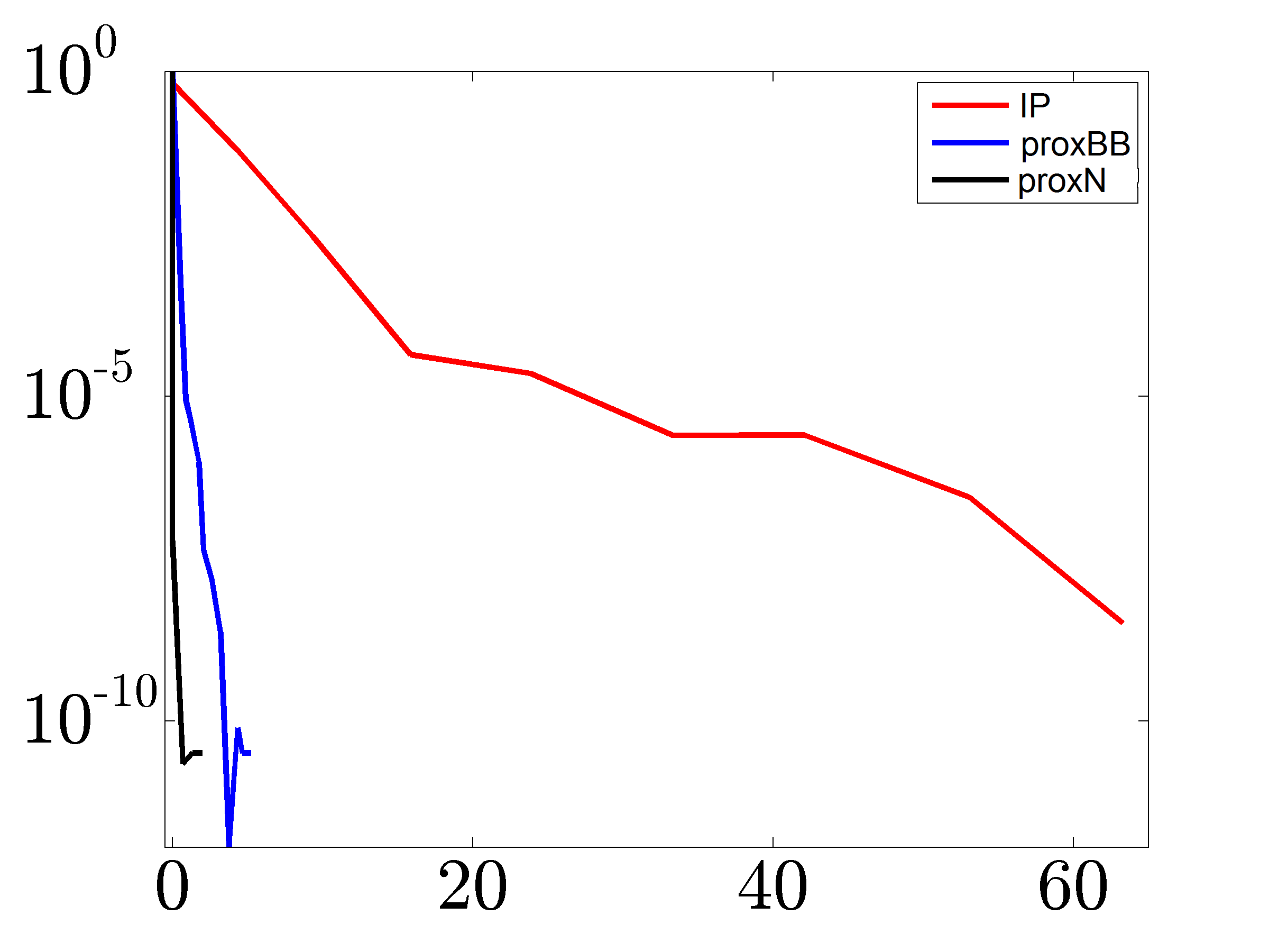
Alternative performance criterion
We next use our customized algorithms for adding edges to an Erdos-Renyi
network with  nodes and
  edges in the controller graph.
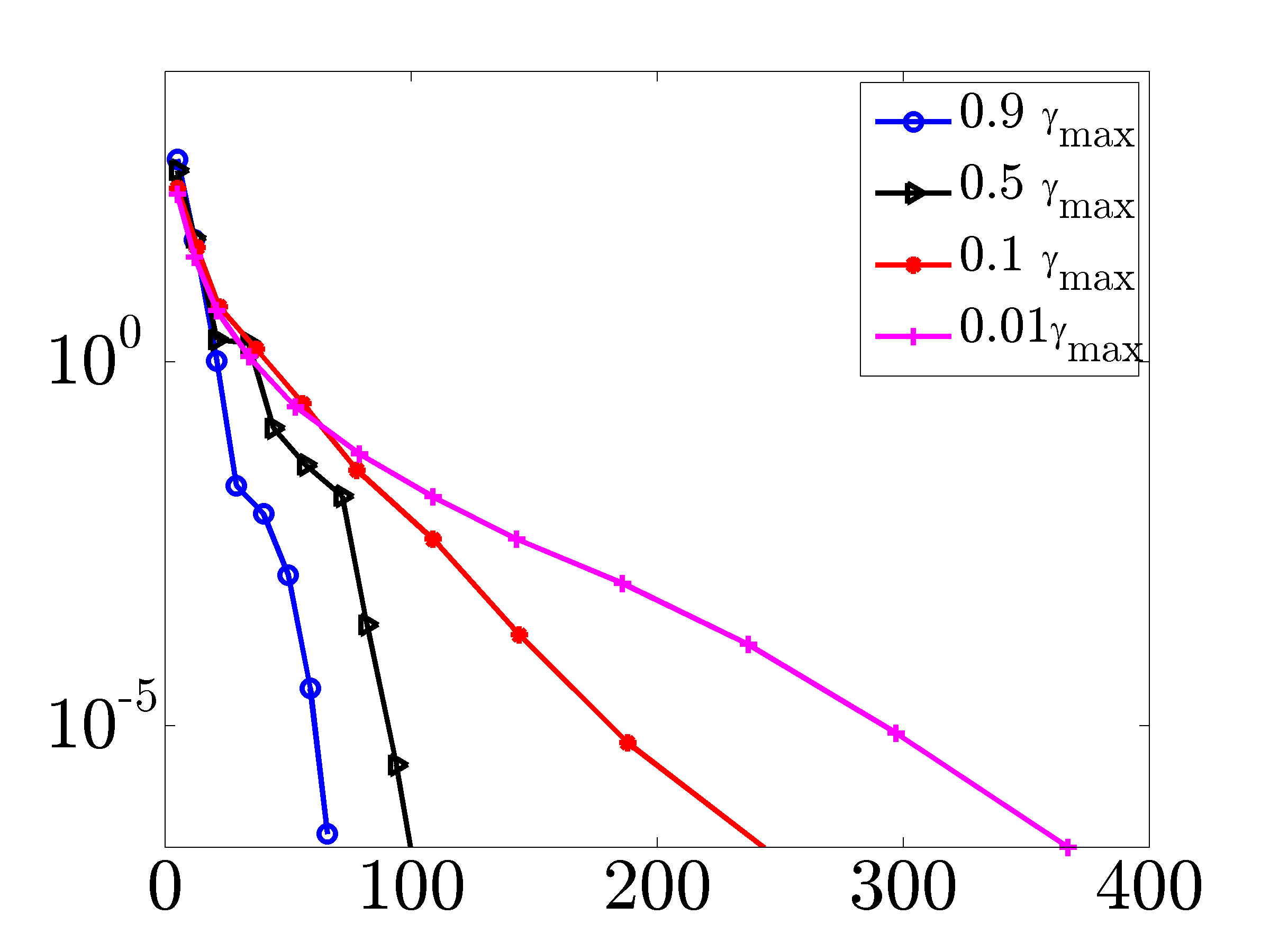
The following shows the relative error in the objective function in
logarithmic scale versus the computation time. Here,
edges in the controller graph.
The following shows the relative error in the objective function in
logarithmic scale versus the computation time. Here,  is the optimal
vector of the edge weights obtained using primal-dual interior point method.
We set the tolerances for and to and ,
respectively. Even for a problem of relatively small size, both proxN and
proxBB converge much faster than the IP algorithm and proxN outperforms
proxBB.
is the optimal
vector of the edge weights obtained using primal-dual interior point method.
We set the tolerances for and to and ,
respectively. Even for a problem of relatively small size, both proxN and
proxBB converge much faster than the IP algorithm and proxN outperforms
proxBB.
Thus, a possible less sophisticated criterion for termination is the relative
change in the objective function value,
 We have examined this criterion for our customized algorithm. Not only
did not we encounter false termination but also the accuracy of the obtained
solutions were very high. However, for a fair comparison with IP algorithm,
we report the results using the generic stopping criteria in Remarks
We have examined this criterion for our customized algorithm. Not only
did not we encounter false termination but also the accuracy of the obtained
solutions were very high. However, for a fair comparison with IP algorithm,
we report the results using the generic stopping criteria in Remarks  and
and  .
.
 |
|

Proximal gradient vs fast greedy algorithm
We next compare our proximal gradient algorithm with the fast greedy
algorithm of Summers et al., 2015. We solve problem  for Erdos-Renyi networks with different number of nodes (
 to
to  )
and
)
and  . After proxBB identifies the edges in the
controller graph, we use the greedy method to select the same number of
edges. Finally, we polish the identified edge weights for both methods.
. After proxBB identifies the edges in the
controller graph, we use the greedy method to select the same number of
edges. Finally, we polish the identified edge weights for both methods.
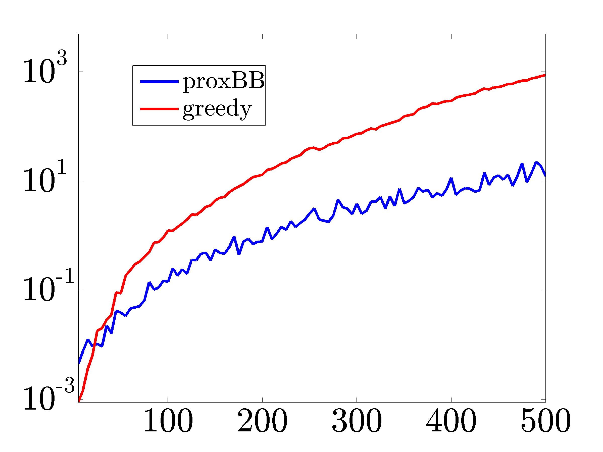 |
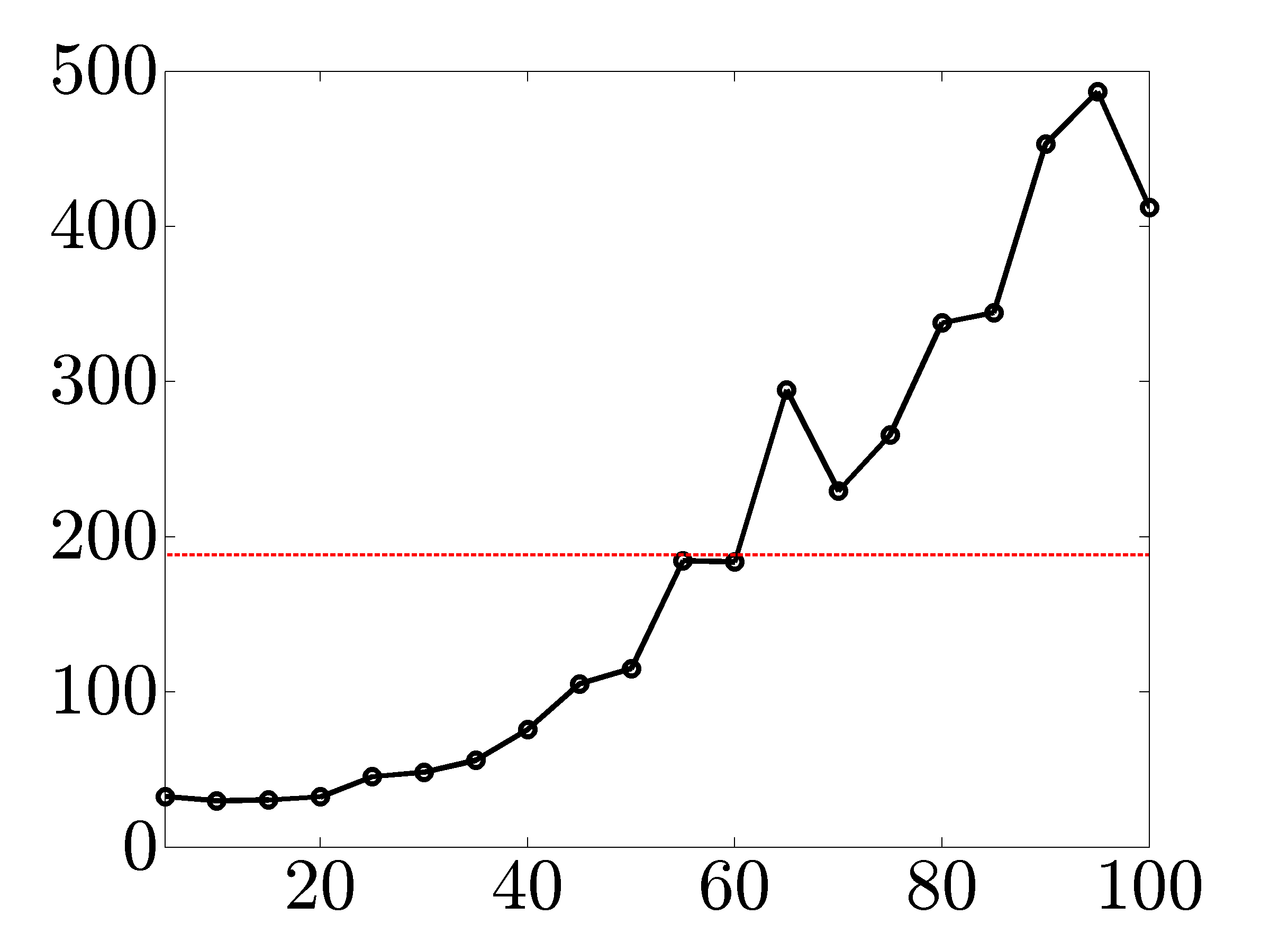
The solve times (in seconds) versus the number of nodes. As the number of nodes increases the proximal gradient algorithm significantly outperforms the fast greedy method. |

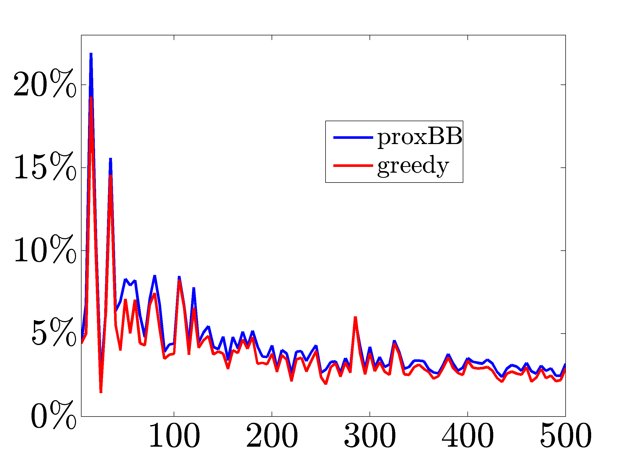 |
Relative to the optimal centralized controller, both methods yield similar performance degradation of the closed-loop network. |