Disconnected plant network
The following example was originally studied in the
PhD
Dissertation of Fu Lin. The plant graph
contains  randomly distributed nodes in a region of
  units. Two nodes are neighbors if their Euclidean distance is not greater
than
units. Two nodes are neighbors if their Euclidean distance is not greater
than  units. We examine the problem of adding edges to a plant graph
which is not connected and solve the sparsity-promoting optimal control
problem (P) using graphsp_IP_w.m for controller graph with
units. We examine the problem of adding edges to a plant graph
which is not connected and solve the sparsity-promoting optimal control
problem (P) using graphsp_IP_w.m for controller graph with  potential edges. This is done for
  logarithmically-spaced values of
![gamma in [10^{-3},2.5]](eqs/1661114254-130.png) using the path-following iterative reweighted
algorithm that employs the weighted
using the path-following iterative reweighted
algorithm that employs the weighted  norm as a proxy for inducing
sparsity
norm as a proxy for inducing
sparsity
Following Candes,
Wakin, and Boyd ’08, we set the weights  to be inversely proportional
to the magnitude of the solution
to be inversely proportional
to the magnitude of the solution  to (SP) at the previous value of
 ,
,
where  is introduced to ensure that the weights are
well-defined when
is introduced to ensure that the weights are
well-defined when  . For
. For  , we initialize weights
using the optimal centralized vector of the edge weights
, we initialize weights
using the optimal centralized vector of the edge weights  . Topology
identification is followed by the polishing step that computes the optimal
vector of the controller edge weights.
. Topology
identification is followed by the polishing step that computes the optimal
vector of the controller edge weights.
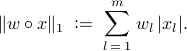
The optimal centralized vector of the edge weights contains both
negative and positive elements.
 |
The optimal centralized vector of the edge weights |
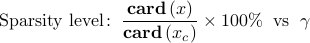
The number of nonzero elements in the vector of the controller edge weights
decreases and the closed-loop performance deteriorates as
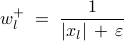
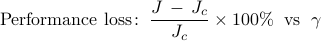
increases. In particular, we show the optimal tradeoff curve between the
 performance loss (relative to the optimal centralized
controller) and the sparsity of the vector .
performance loss (relative to the optimal centralized
controller) and the sparsity of the vector .
 |
For Increased emphasis on sparsity induces controller graphs with smaller number of nonzero elements. |
 |
Relative to the optimal centralized controller, performance of the optimal sparse controller deteriorates gracefully with increased emphasis on sparsity. |
 |
The optimal tradeoff curve between the |

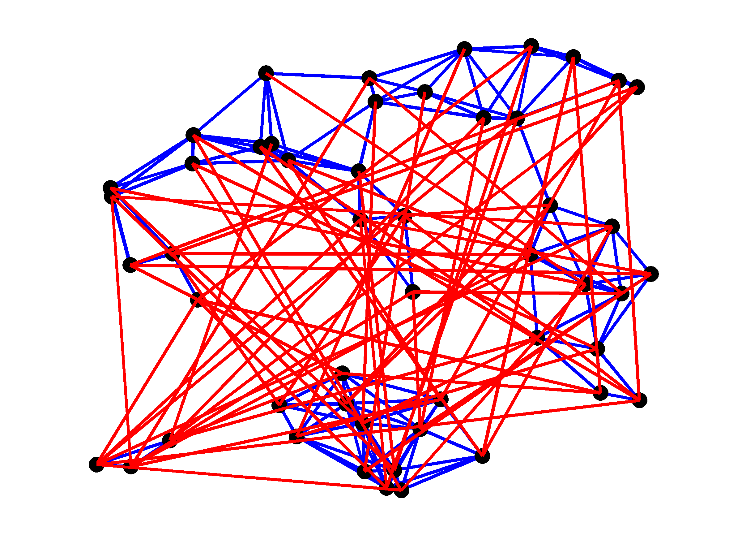
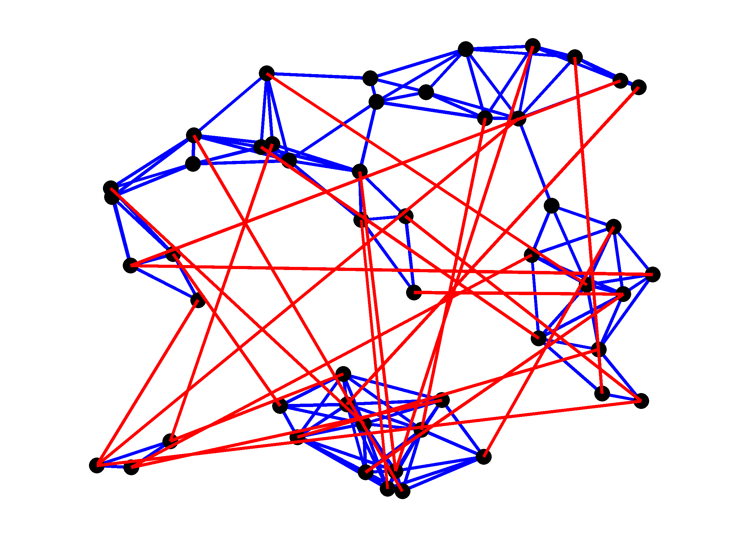
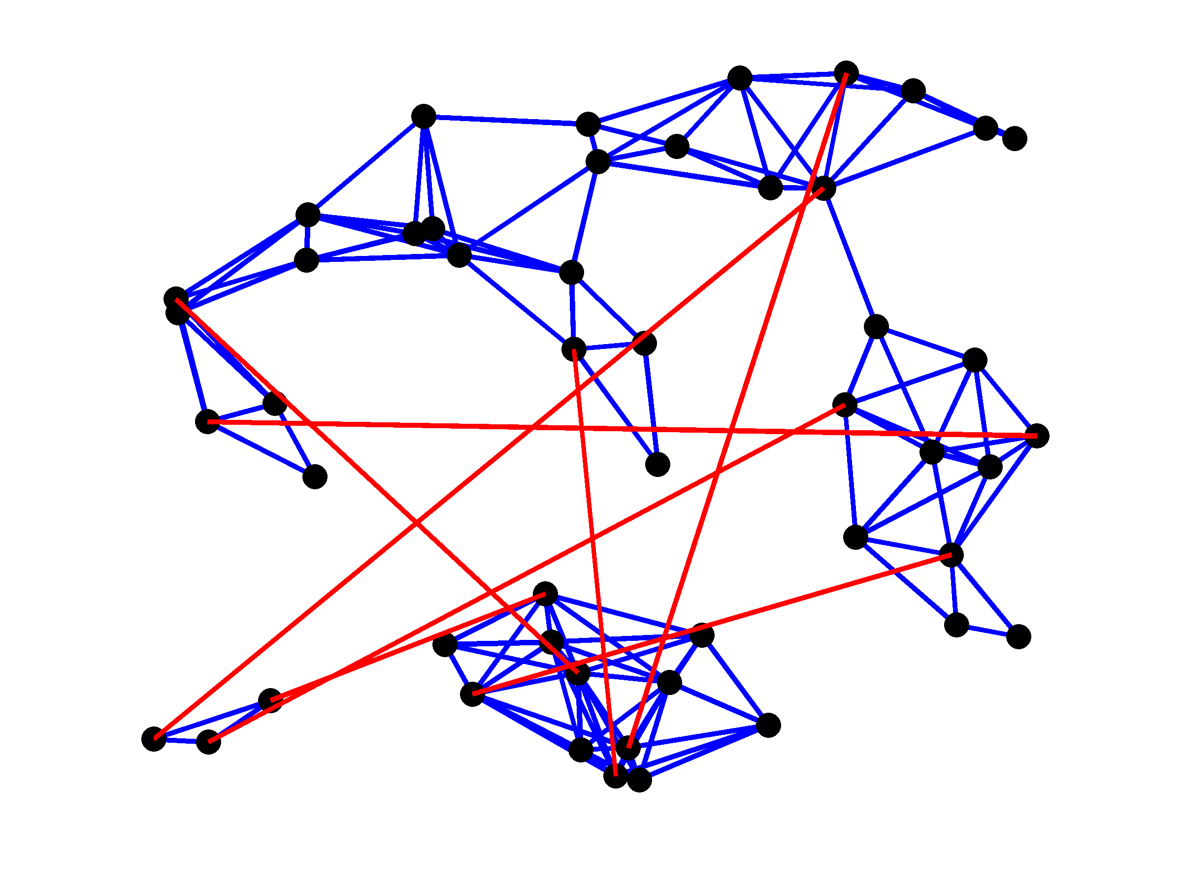
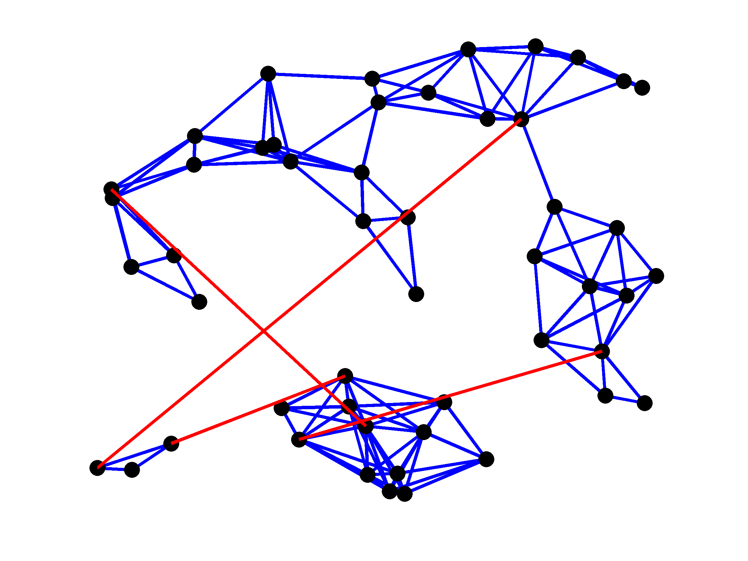
Topologies of the plant (blue lines) and controller graphs (red lines) for
four values of . As expected, larger values of yield
sparser controller graphs. Since the plant graph has three disconnected
subgraphs, at least two edges in the controller are needed to make the
closed-loop network connected.
 |
|

 |
|

 |
|

 |
|
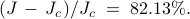
For  , only four edges are added. Relative to the optimal
centralized vector of the controller edge weights , the identified
sparse controller in this case uses only
, only four edges are added. Relative to the optimal
centralized vector of the controller edge weights , the identified
sparse controller in this case uses only  of the edges, i.e.,

and achieves a performance loss of  ,
,
Here, is the solution to (P) with  and the pattern of
non-zero elements of is obtained by solving (P) with
via the path-following iterative reweighted algorithm.
and the pattern of
non-zero elements of is obtained by solving (P) with
via the path-following iterative reweighted algorithm.