DMDSP – Sparsity-Promoting Dynamic Mode Decomposition

Mihailo R. Jovanovic, Peter J. Schmid, Joseph W. Nichols September 2013 Matlab Files Download all Matlab files Presentation 2013 SIAM Talk Paper 2014 Physics of Fluids Paper

Purpose

This website provides a Matlab implementation of the Sparsity-Promoting Dynamic Mode Decomposition (DMDSP) algorithm. Dynamic Mode Decomposition (DMD) is an effective means for capturing the essential features of numerically or experimentally generated snapshots, and its sparsity-promoting variant DMDSP achieves a desirable tradeoff between the quality of approximation (in the least-squares sense) and the number of modes that are used to approximate available data. Sparsity is induced by augmenting the least-squares deviation between the matrix of snapshots and the linear combination of DMD modes with an additional term that penalizes the -norm of the vector of DMD amplitudes. We employ alternating direction method of multipliers (ADMM) to solve the resulting convex optimization problem and to efficiently compute the globally optimal solution.

Problem formulation

Dynamic Mode Decomposition

Starting with a sequence of snapshots

DMD provides a low-dimensional representation of a discrete-time linear time-invariant system

on a subspace spanned by the basis resulting from the Proper Orthogonal Decomposion (POD) of the data sequence. In particular, given two data matrices

the DMD algorithm provides optimal representation of the matrix in the basis spanned by the POD modes of ,

Here, is the rank of the matrix of snapshots , and is the complex-conjugate-transpose of the matrix of POD modes which is obtained from an economy-size singular value decomposition (SVD) of ,

where is an diagonal matrix determined by the non-zero singular values of , and

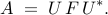
The matrix is determined from the matrices of snapshots and by minimizing the Frobenius norm of the difference between and , thereby resulting into

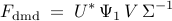
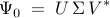
Optimal amplitudes of DMD modes

The matrix determines an optimal low-dimensional representation of the inter-snapshot mapping on the subspace spanned by the POD modes of . The dynamics on this -dimensional subspace are governed by

and the matrix of POD modes can be used to map into a higher dimensional space ,

If has a full set of linearly independent eigenvectors , with corresponding eigenvalues , then it can be brought into a diagonal coordinate form and experimental or numerical snapshots can be approximated using a linear combination of DMD modes,

or, equivalently, in matrix form,

Here, the matrix of POD modes and the matrix of eigenvectors of , are used to determine the matrix of DMD modes

Furthermore, the amplitude quantifies the th modal contribution of the initial condition on the subspace spanned by the POD modes of , and the temporal evolution of the dynamic modes is governed by the Vandermonde matrix which is determined by the eigenvalues of .

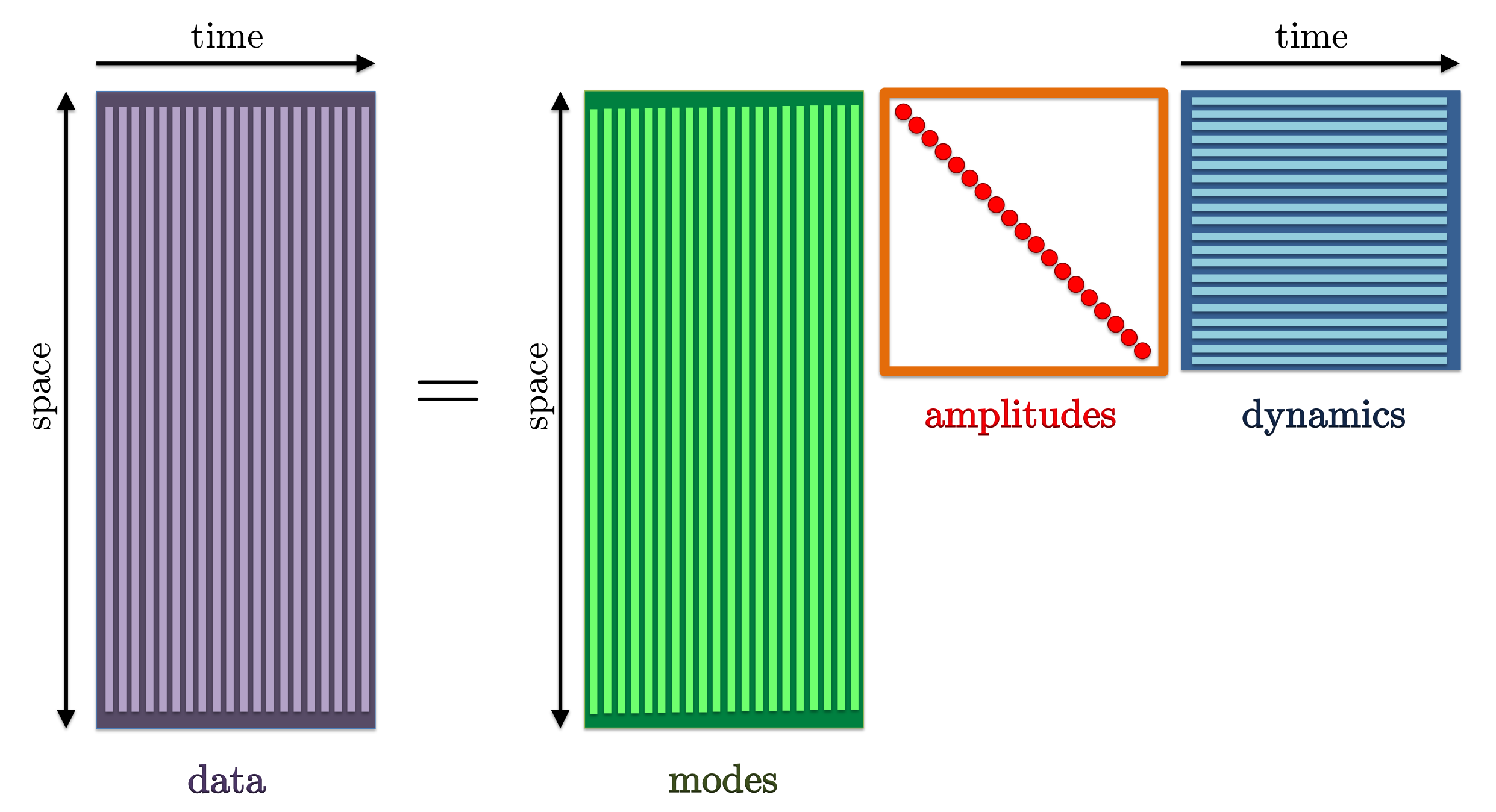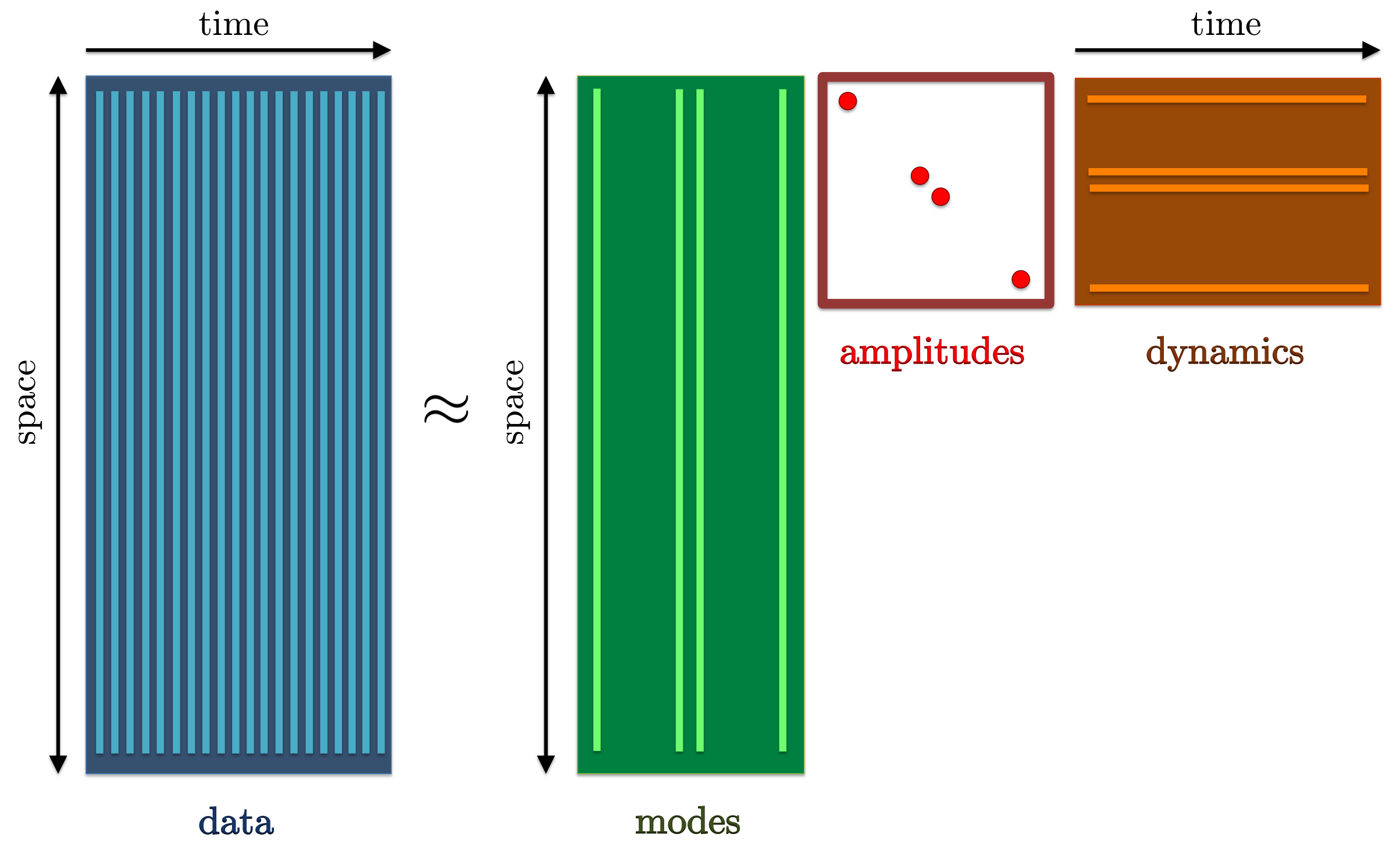
Dynamic mode decomposition can be used to represent experimentally or numerically generated snapshots as a linear combination of DMD modes, properly weighted by their amplitudes and advanced in time according to their temporal growth/decay rate.

Determination of the optimal vector of amplitudes then amounts to minimization of the Frobenius norm of the difference between and . Using SVD of the definition of the matrix , and a sequence of straightforward algebraic manipulations, this convex optimization problem can be brought into the following form

where is the optimization variable and the problem data is determined by

Here, an asterisk denotes the complex-conjugate-transpose of a vector (matrix), an overline signifies the complex-conjugate of a vector (matrix), of a vector is a diagonal matrix with its main diagonal determined by the elements of a given vector, of a matrix is a vector determined by the main diagonal of a given matrix, and is the elementwise multiplication of two matrices.

The optimal vector of DMD amplitudes that minimizes the Frobenius norm of the difference between and can thus be obtained by minimizing the quadratic function with respect to ,

Sparsity-promoting dynamic mode decomposition

We now direct our attention to the problem of selecting the subset of DMD modes that has the most profound influence on the quality of approximation of a given sequence of snapshots. In the first step, we seek a sparsity structure that achieves a user-defined tradeoff between the number of extracted modes and the approximation error (with respect to the full data sequence). In the second step, we fix the sparsity structure of the vector of amplitudes (identified in the first step) and determine the optimal values of the non-zero amplitudes.

The sparsity-promoting dynamic mode decomposition is aimed at identifying a subset of DMD modes that optimally approximate the entire data sequence.

We approach the problem of inducing sparsity by augmenting the objective function with an additional term that penalizes the the -norm of the vector of unknown amplitudes ,

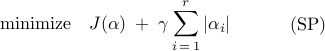
In the modified optimization problem (SP), is a positive regularization parameter that reflects our emphasis on sparsity of the vector . Larger values of place stronger emphasis on the number of non-zero elements in the vector (relative to the quality of the least-squares approximation, ), thereby encouraging sparser solutions.

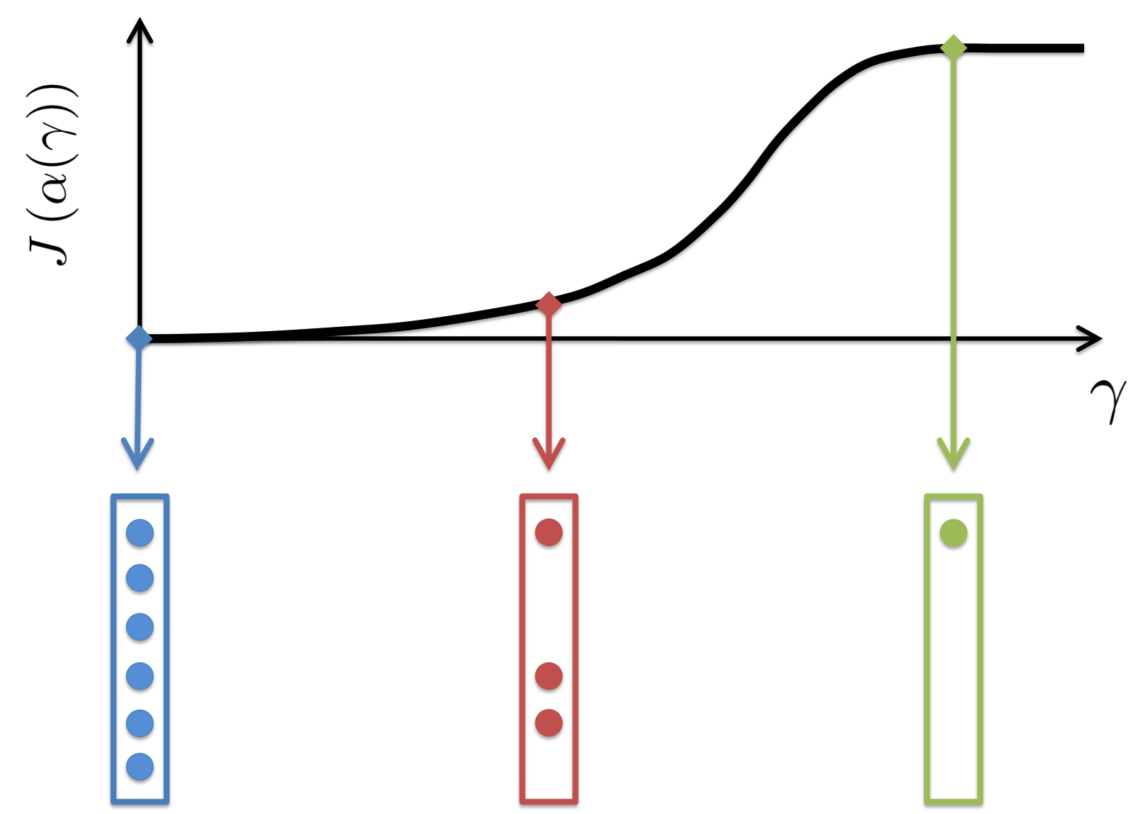Increased emphasis on sparsity encourages sparser solutions at the expense of compromising quality of least-squares approximation.

After a desired balance between the quality of approximation of experimental or numerical snapshots and the number of DMD modes is achieved, we fix the sparsity structure of the unknown vector of amplitudes and determine only the non-zero amplitudes as the solution to the following constrained convex optimization problem:

Here, the matrix encodes information about the sparsity structure of the vector . The columns of are the unit vectors in whose non-zero elements correspond to zero components of . For example, for with

the matrix is given as

Alternating direction method of multipliers (ADMM)

ADMM is a simple but powerful algorithm well-suited to large optimization problems. In the sparsity-promoting DMD problem, the algorithm consists of four steps:

• Step 1: introduce additional variable/constraint

• Step 2: introduce the augmented Lagrangian

• Step 3: use ADMM for the augmented Lagrangian minimization

• Step 4: polishing - solve the structured quadratic programming problem for the identified sparsity pattern

Solution to (SP)

The respective structures of the functions and in the sparsity-promoting DMD problem can be exploited to show that the -minimization step amounts to solving an unconstrained regularized quadratic program and that the -minimization step amounts to a use of the soft thresholding operator :

where

Solution to (POL)

After the desired sparsity structure has been identified, the optimal vector of amplitudes with a fixed sparsity structure, , can be determined from:

Acknowledgments

We gratefully acknowledge Prof. Parviz Moin for his encouragement to pursue this effort during the 2012 Center for Turbulence Research Summer Program at Stanford University.