Two-dimensional channel flow
(Orr-Sommerfeld operator)

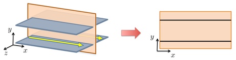Two-dimensional channel flow geometry.

The Orr-Sommerfeld equation governs the dynamics of two-dimensional velocity fluctuations around the laminar channel flow,

$begin{array}{rcl} Delta phi_{t} (k_x, y, t) & !! = !! & left( {displaystyle frac{1}{R}} Delta^{2} , - , mathrm{i} , k_x , U(y) , Delta , + , mathrm{i} , k_x , U''(y) right) phi(k_x, y, t) [0.3cm] & & + , D^{(1)} , d_{1}(k_x, y, t) , - , mathrm{i} , k_x , d_{2}(k_x, y, t), ;;; y in left[ -1, 1 right] end{array}$

where

	—	streamfunction
,	—	streamwise and wall-normal forcing
	—	Reynolds number
	—	streamwise wavenumber
	—	for shear-driven flow
	—	for pressure-driven flow
$Delta = D^{(2)} - k_x^2$	—	Laplacian
$Delta^2 = D^{(4)} - 2 , k_x^2 , D^{(2)} + k_x^4$ .

The boundary conditions are given by

$phi(k_x, pm 1, t) ; = ; D^{(1)} phi(k_x, pm 1, t) ; = ; 0.$

The desired outputs are the streamwise and wall-normal velocity fluctuations,

$begin{array}{rcl} u(k_x, y, t) & !! = !! & D^{(1)} , phi(k_x, y, t) [0.15cm] v(k_x, y, t) & !! = !! & -mathrm{i} , k_x , phi(k_x, y, t). end{array}$

The input-output differential equation representing the frequency response operator is given by

$left( {displaystyle frac{1}{R}} D^{(4)} , + , a_{2}(y) , D^{(2)} , + , a_{0}(y) right) phi(y) ; = ; -D^{(1)} , d_{1}(y) , + , mathrm{i} , k_x , d_{2}(y)$

where

$begin{array}{rcl} a_{2}(y) & !! = !! & {displaystyle -left( frac{2 , k_x^2}{R} , + , mathrm{i}, k_x , U(y) , + , mathrm{i} , omega right)} [0.4cm] a_{0}(y) & !! = !! & {displaystyle frac{k_x^{4}}{R}} , + , mathrm{i} , k_x^3 , U(y) , + , mathrm{i} , k_x , U''(y) , + , mathrm{i} , omega , k_x^2. end{array}$

Matlab codes

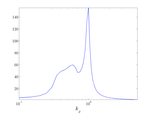
Find the largest singular value of the frequency response operator for the Orr-Sommerfeld equation in a pressure-driven channel flow as a function of k_x at omega = -0.3 .

% System parameters:

R = 2000; % Reynolds number

kxval = linspace(0.1,5,100); % streamwise wave-number
kxgrd = length(kxval);

om = -0.3; % temporal frequency

dom = domain(-1,1);     % domain of your function
y = chebfun('y',dom);
fone = chebfun(1,dom);      % fone(y) = 1
fzero = chebfun(0,dom);     % fzero(y) = 0

U = diag(1 - y.^2);    % in pressure-driven flow
Uy = diag(-2*y);
Uyy = diag(-2*fone);

% Boundary conditions
Wa0{1} = [1, 0, 0, 0; 0, 1, 0, 0];
Wb0{1} = [1, 0, 0, 0; 0, 1, 0, 0];

% Looping over different values of kx
Smax = zeros(kxgrd,1); A0 = cell(1,1); B0 = cell(1,2); C0 = cell(2,1);

for indx = 1:kxgrd

    kx = kxval(indx); kx2 = kx*kx; kx4 = kx2*kx2;

    % coefficients of the A0 operator
    % a0*phi + 0*phi' + a2*phi'' + 0*phi''' + 1/R*phi''''
    a2 = -(2*kx2*(1/R)*fone + 1i*kx*U*fone + 1i*om*fone);
    a0 = (1/R)*kx4*fone + 1i*kx*kx2*U*fone + 1i*kx*Uyy*fone + ...
        1i*om*kx2*fone;

    A0{1} = [a0, fzero, a2, fzero, (1/R)*fone];

    % coefficients of the B0 operator
    % 0*d1 - d1' + i*kx*d2 + 0*d2'
    B0{1,1} = [fzero, -fone]; B0{1,2} = [1i*kx*fone, fzero];

    % coefficients of the C0 operator
    % u = 0*phi + 1*phi'; v = -i*kx*phi + 0*phi'
    C0{1,1} = [fzero, fone]; C0{2,1} = [-1i*kx*fone, fzero];

    % solving for the left principal singular pair
    [Sfun, Sval] = svdfr(A0,B0,C0,Wa0,Wb0,1,1);

    % saving the largest singular value at each kx
    Smax(indx) = Sval(1);

end

% Plotting the largest singular value as a function of kx at a fixed om
plot(kxval,Smax,'-','LineWidth',1.1);
xlab = xlabel('k_x', 'interpreter', 'tex');
set(xlab, 'FontName', 'cmmi10', 'FontSize', 20);
h = get(gcf,'CurrentAxes');
set(h,'FontName','cmr10','FontSize',15,'xscale','log','yscale','lin');

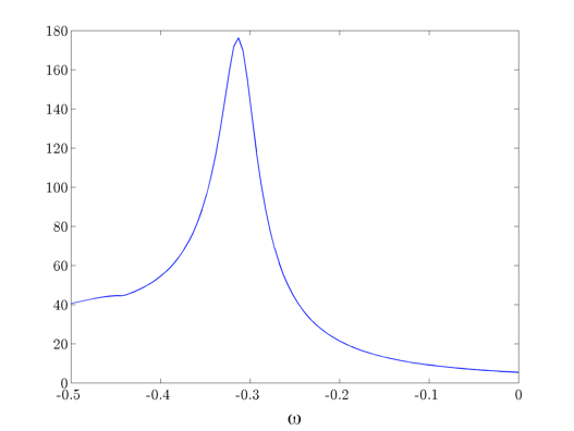
Find the largest singular value of the frequency response operator for the Orr-Sommerfeld equation in a pressure-driven channel flow as a function of omega at k_x = 1 .

% the OS-equation as a function of om at kx = 1.
% System parameters:
kx = 1; % streamwise wave-number
kx2 = kx*kx; kx4 = kx2*kx2;

omval = linspace(-0.5,0,100); % temporal frequency
omgrd = length(omval);

% Looping over different values of om
Smax = zeros(omgrd,1); A0 = cell(1,1); B0 = cell(1,2); C0 = cell(2,1);

for indom = 1:omgrd

    om = omval(indom);

    % coefficients of the A0 operator
    % a0*phi + 0*phi' + a2*phi'' + 0*phi''' + 1/R*phi''''
    a2 = -(2*kx2*(1/R)*fone + 1i*kx*U*fone + 1i*om*fone);
    a0 = (1/R)*kx4*fone + 1i*kx*kx2*U*fone + 1i*kx*Uyy*fone + ...
        1i*om*kx2*fone;

    A0{1} = [a0, fzero, a2, fzero, (1/R)*fone];

    % coefficients of the B0 operator
    % 0*d1 - 1*d1' + i*kx*d2 + 0*d2'
    B0{1,1} = [fzero, -fone]; B0{1,2} = [1i*kx*fone, fzero];

    % coefficients of the C0 operator
    % u = 0*phi + 1*phi'; v = -i*kx*phi + 0*phi'
    C0{1,1} = [fzero, fone]; C0{2,1} = [-1i*kx*fone, fzero];

    % solving for the left principal singular pair
    [Sfun, Sval] = svdfr(A0,B0,C0,Wa0,Wb0,1,1);

    % saving the largest singular value for each value of om
    Smax(indom) = Sval(1);

end

% Plotting the largest singular value as a function of om at a fixed kx
plot(omval,Smax,'-','LineWidth',1.1);
xlab = xlabel('\omega', 'interpreter', 'tex');
set(xlab, 'FontName', 'cmmi10', 'FontSize', 20);
h = get(gcf,'CurrentAxes');
set(h,'FontName','cmr10','FontSize',15,'xscale','lin','yscale','lin');

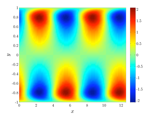
Find the most amplified flow structures for the Orr-Sommerfeld equation in a pressure-driven channel flow at k_x = 1 and omega = -0.313 .

% System parameters:
kxval = [1 -1];   % streamwise wave-number
omval  = 0.313*[-1 1]; % temporal frequency

N = 100;    % number of collocation points for plotting
yd = chebpts(N);

% Looping over different values of om and kx
A0 = cell(1,1); B0 = cell(1,2); C0 = cell(2,1);

for n = 1:2

    om = omval(n);
    kx = kxval(n); kx2 = kx*kx; kx4 = kx2*kx2;

    % coefficients of the A0 operator
    % a0*phi + 0*phi' + a2*phi'' + 0*phi''' + 1/R*phi''''
    a2 = -(2*kx2*(1/R)*fone + 1i*kx*U*fone + 1i*om*fone);
    a0 = (1/R)*kx4*fone + 1i*kx*kx2*U*fone + 1i*kx*Uyy*fone + ...
        1i*om*kx2*fone;

    A0{1} = [a0, fzero, a2, fzero, (1/R)*fone];

    % coefficients of the B0 operator
    % 0*d1 - 1*d1' + i*kx*d2 + 0*d2'
    B0{1,1} = [fzero, -fone]; B0{1,2} = [1i*kx*fone, fzero];

    % coefficients of the C0 operator
    % u = 0*phi + 1*phi'; v = -i*kx*phi + 0*phi'
    C0{1,1} = [fzero, fone]; C0{2,1} = [-1i*kx*fone, fzero];

    % solving for the left principal singular pair
    [Sfun, Sval] = svdfr(A0,B0,C0,Wa0,Wb0,1,1);

    ui = Sfun{1}; % streamwise velocity
    vi = Sfun{2}; % wall-normal velocity

    % discretized values for plotting
    uvec(:,n) = ui(yd,1); vvec(:,n) = vi(yd,1);

end

% Getting physical fields of u and v
kx = abs(kxval(1));
xval = linspace(0, 4*pi/kx, 100); % streamwise coordinate

Up = zeros(N,length(xval));   % physical value of u
Vp = zeros(N,length(xval));   % physical value of v

for indx = 1:length(xval)

    x = xval(indx);

    for n = 1:2

        kx = kxval(n);

        Up(:,indx) =  Up(:,indx) + uvec(:,n)*exp(1i*kx*x);
        Vp(:,indx) =  Vp(:,indx) + vvec(:,n)*exp(1i*kx*x);

    end

end

Up = real(Up); Vp = real(Vp); % only real part exists

% Plotting the most amplified streamwise velocity structures
pcolor(xval,yd,Up); shading interp;
cb = colorbar('vert');
xlab = xlabel('x', 'interpreter', 'tex');
ylab = ylabel('y', 'interpreter', 'tex');
set(xlab, 'FontName', 'cmmi10', 'FontSize', 20);
set(ylab, 'FontName', 'cmmi10', 'FontSize', 20);
h = get(gcf,'CurrentAxes');
set(h,'FontName','cmr10','FontSize',15,'xscale','lin','yscale','lin');
set(cb, 'FontName', 'cmr10', 'FontSize', 15);

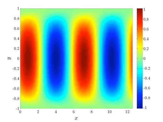
Plot the most amplified wall-normal velocity structures.

pcolor(xval,yd,Vp); shading interp;
cb = colorbar('vert');
xlab = xlabel('x', 'interpreter', 'tex');
ylab = ylabel('y', 'interpreter', 'tex');
set(xlab, 'FontName', 'cmmi10', 'FontSize', 20);
set(ylab, 'FontName', 'cmmi10', 'FontSize', 20);
h = get(gcf,'CurrentAxes');
set(h,'FontName','cmr10','FontSize',15,'xscale','lin','yscale','lin');
set(cb, 'FontName', 'cmr10', 'FontSize', 15);

Two-dimensional channel flow (Orr-Sommerfeld operator)

Matlab codes

Two-dimensional channel flow
(Orr-Sommerfeld operator)