Mass-spring-damper system

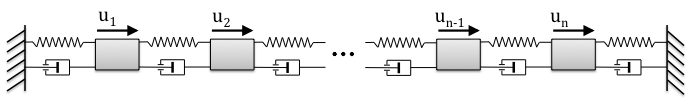For a stochastically-forced mass-spring-damper system with masses on a line with state-space representation

$dot{x} ;=; A,x ;+; B_u, u$

the state vector is determined by x = [,p^T, ~, v^T ,]^T and contains the position and velocity of all masses. The state and input matrices are

$A ;=; left[ begin{array}{cc} O & I -T & -I end{array} right],~~~~ B_u ;=; left[ begin{array}{c} O I end{array} right]$

where and are zero and identity matrices of suitable sizes, and is a symmetric tridiagonal Toeplitz matrix with on the main diagonal and on the first upper and lower sub-diagonals. Stochastic disturbances are generated by a low-pass filter

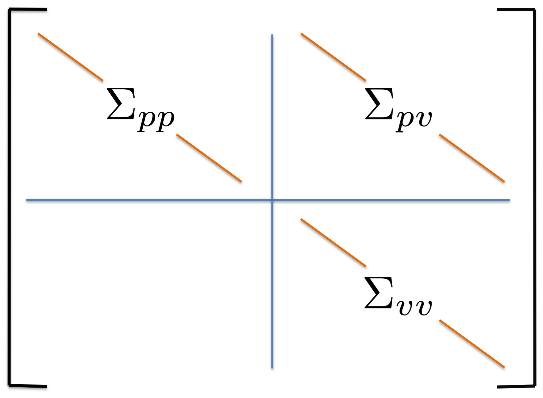
where represents a zero-mean unit variance white process. The steady-state covariance of the of the stochastically-forced mass-spring-damper system can be extracted from the steady-state covariance of the cascade of filter and system dynamics, and is partitioned as

$Sigma_{xx} ;=; left[ begin{array}{cc} Sigma_{pp} & Sigma_{pv} Sigma_{vp} & Sigma_{vv} end{array} right]$

We assume knowledge of one-point correlations of the position and velocity of
masses, i.e., the diagonal elements of matrices $Sigma_{pp}$ , $Sigma_{vv}$ , and $Sigma_{pv}$ , which are
shown as orange lines in the figure. It is desired to identify the suitable forcing
model which accounts for the available and completes the unavailable
second-order statistics in .

Performance comparison

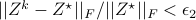The following table compares solve times of CVX and the customized algorithms discussed in the paper. Each method stops when an iterate achieves a certain distance from optimality, i.e., ||X^k-X^star||_F/ ||X^star||_F < epsilon_1 and ||Z^k-Z^star||_F/ ||Z^star||_F < epsilon_2 . The choice of epsilon_1, epsilon_2 = 0.01 , guarantees that the primal objective is within 0.1% of J_p(X^star,Z^star) . For n=50 and n=100 , CVX ran out of memory. Clearly, for large problems, AMA with BB step-size initialization significantly outperforms both regular AMA and ADMM.

								$bf{AMA_{BB}}$

Convergence curves showing the performance of the customized AMA
with (-) and without ( triangle ) BB step-size initialization and ADMM ( circ )
for the mass-spring-damper system with masses and gamma=2.2 . Here,
J_d^star is the optimal dual objective.

Quality of completion and verification in linear stochastic simulations

For gamma=2.2 , the spectrum of contains positive and negative eigenvalues. Based on Proposition of the paper, can be decomposed into B H^*+ H B^* , where has independent columns. In other words, the identified can be explained by driving the state-space model with stochastic inputs . Based on this, we construct the optimal filter that generates the suitable stochastic input and conduct linear stochastic simulations of the filter dynamics with zero-mean unit variance input to validate our modeling approach.

For gamma = 2.2 , the matrix which results from solving problem (CC)
has a clear-cut in its singular values with of them being nonzero.

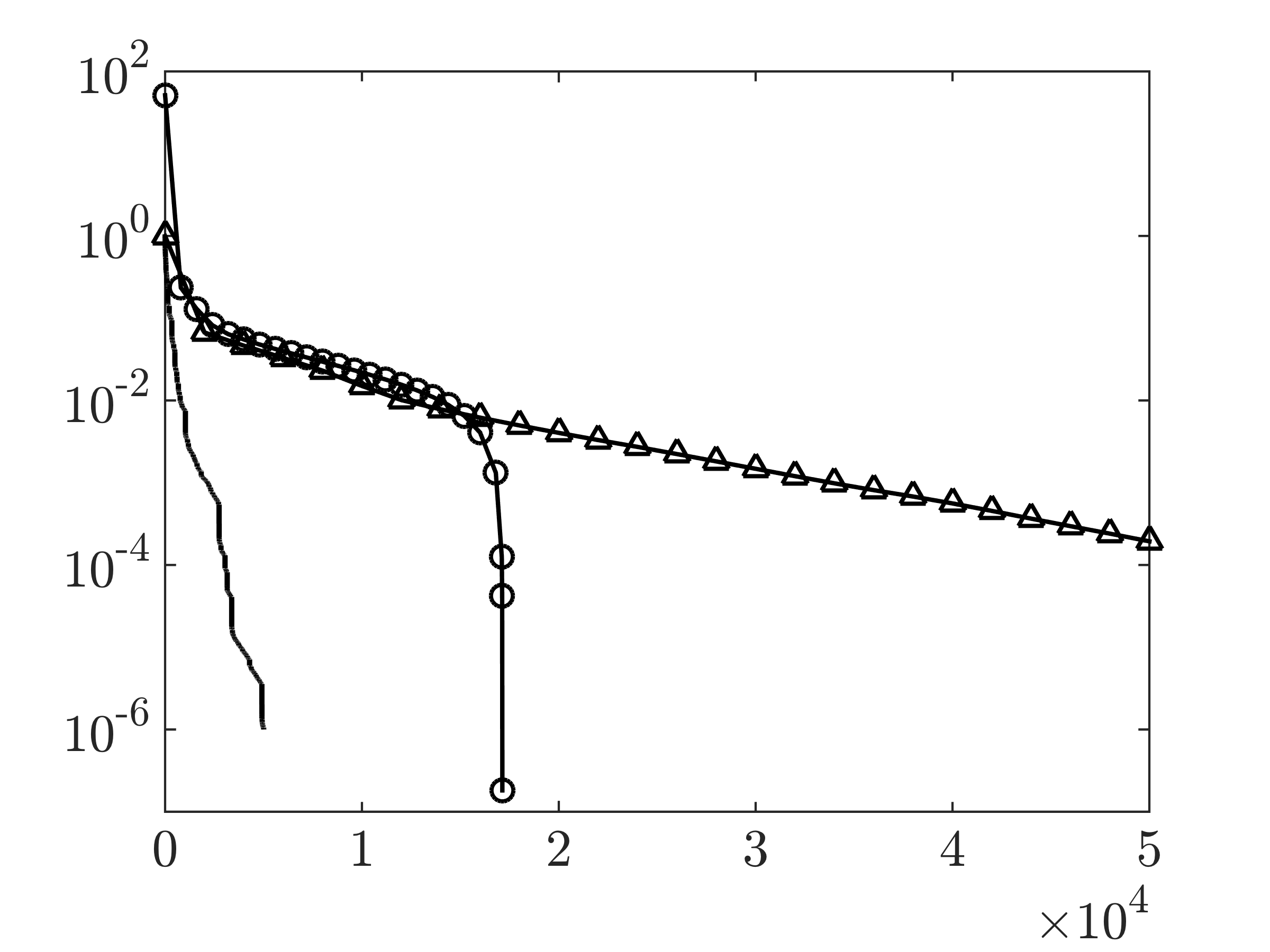
Diagonals of position (left) and velocity
(right) covariances for the mass-spring-
damper system with masses; Solid
black lines show diagonals of $Sigma_{xx}$ and
red circles mark solutions of
optimization problem (CC).

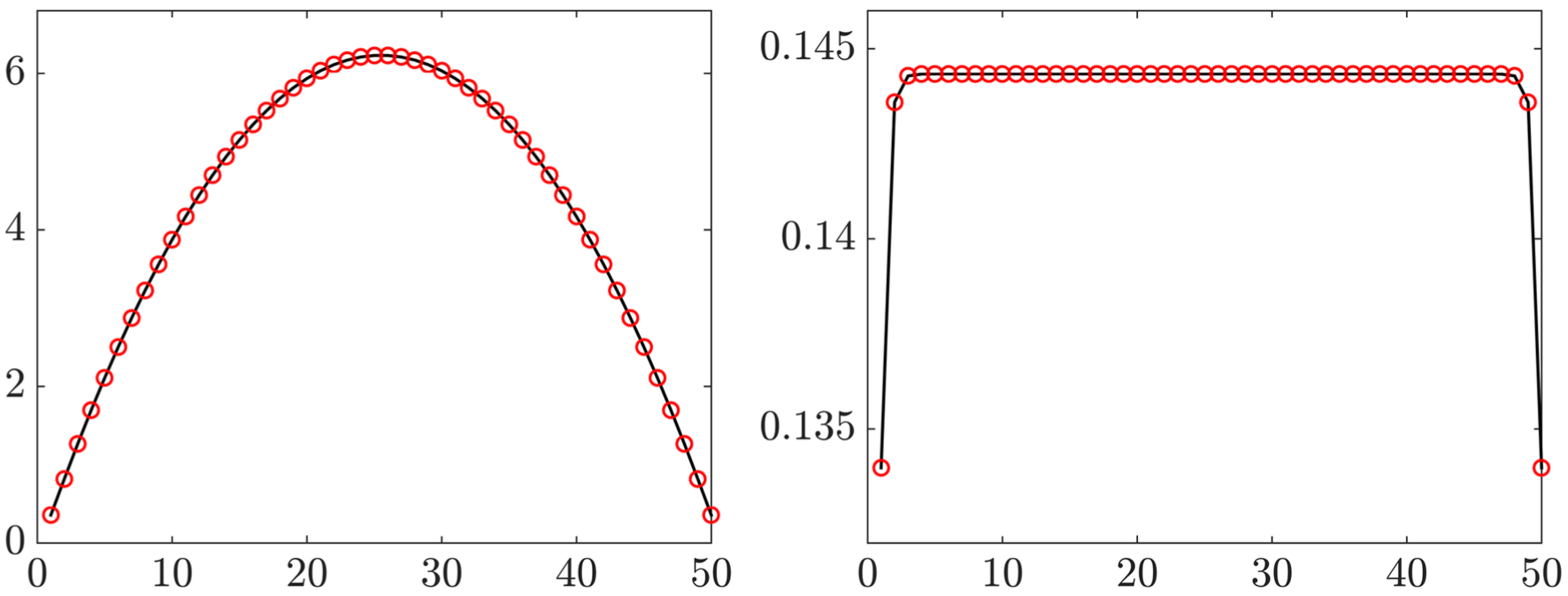
The true covariance $Sigma_{pp}$ of the
mass-spring-damper system (left) and
the recovered covariance matrix $X_{pp}$
resulting from the ensemble-averaged
simulations (right). We note that (i) only
diagonal elements of this matrix (marked
by the black line) are used as data in
optimization problem (CC), and that
(ii) the recovery of the off-diagonal
elements is remarkably consistent.

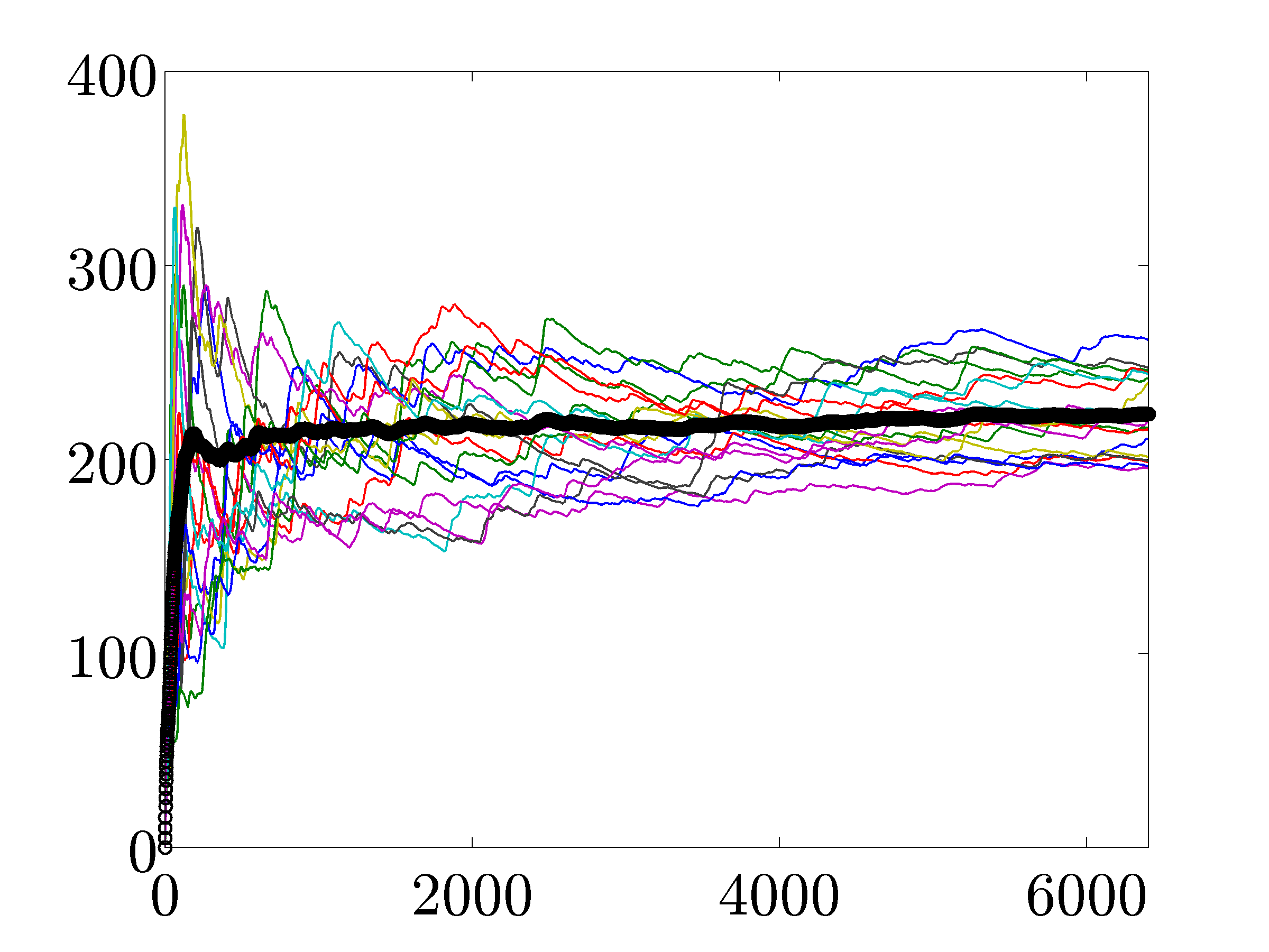Time evolution of the variance of the mass-spring-damper system's
state vector for different realizations of white-in-time forcing to the
filter dynamics. Since proper comparison requires ensemble-averaging,
we have conducted twenty stochastic simulations with different
realizations of the stochastic input. The variance averaged over all
simulations is marked by the thick black line. Even though the
responses of individual simulations differ from each other, the average
of twenty sample sets asymptotically approaches the correct
steady-state variance.