CCAMA – A customized alternating minimization algorithm for structured covariance completion problems
 |
Written by:
April 2016 Matlab Files
Papers
|
Purpose
This website provides a Matlab implementation of a customized alternating minimization algorithm (CCAMA) for solving the covariance completion problem (CC). This problem aims to explain and complete partially available statistical signatures of dynamical systems by identifying the directionality and dynamics of input excitations into linear approximations of the system. In this, we seek to explain correlation data with the least number of possible input disturbance channels. This inverse problem is formulated as a rank minimization, and for its solution, we employ a convex relaxation based on the nuclear norm. CCAMA exploits the structure of (CC) in order to gain computational efficiency and improve scalability.
Problem formulation
Consider a linear time-invariant system
![begin{array}{rcl} dot{x} & !! = !! & A , x ; + ; B , u [0.1cm] y & !! = !! & C, x end{array}](eqs/7622844854399723755-130.png)
where  is the state vector,
  is the output,
  is a
stationary zero-mean stochastic process,
is a
stationary zero-mean stochastic process,  is the dynamic matrix,
  is the input matrix, and
  is the output matrix. For Hurwitz and
controllable
is the output matrix. For Hurwitz and
controllable  , a positive definite matrix
  qualifies as the
steady-state covariance matrix of the state vector
qualifies as the
steady-state covariance matrix of the state vector
if and only if the linear equation

is solvable for  . Here,
  is the expectation operator, represents the cross-correlation of the state
  and the input
  , and
, and  denotes the complex conjugate transpose.
The algebraic relation between second-order statistics of the state and forcing can be used to explain partially known sampled second-order statistics using stochastically-driven LTI systems. While the dynamical generator is known, the origin and directionality of stochastic excitation is unknown. It is also important to restrict the complexity of the forcing model. This complexity is quantified by the number of degrees of freedom that are directly influenced by stochastic forcing and translates into the number of input channels or  . It can be shown that the rank of is closely related to the signature of the matrix
![begin{array}{rcl} Z &!! mathrel{mathop:}= !!& -(A,X ,+, XA^*) [.15cm] &!! = !!& B H^* ,+, H B^*. end{array}](eqs/8015649963986567082-130.png)
The signature of a matrix is determined by the number of its positive, negative, and zero eigenvalues. In addition, the rank of  bounds the rank of .
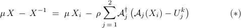
Based on this, the problem of identifying low-complexity structures for stochastic forcing can be formulated as the following structured covariance completion problem
![begin{array}{cl} {rm minimize} & -{rm log,det}left(Xright) ,+, gamma,||Z||_* [.25cm] {rm subject~to} & ~A , X ,+, X A^* ,+, Z ;=; 0 [.15cm] & ,,left(C X C^* right)circ E ,-, G ;=; 0. end{array} hspace{1.5cm} {rm (CC)}](eqs/8909047710954604432-130.png)
Here,  is a positive regularization parameter, the matrices , ,
  , and
, and  are problem data, and the Hermitian matrices , are optimization variables. Entries of represent partially available second-order statistics of the output
  , the symbol
  denotes elementwise matrix multiplication, and is the structural identity matrix,
![E_{ij} ;=; left{ begin{array}{ll} 1, &~ mathrm{if} ~ G_{ij} ~ {rm is~available} [.1cm] 0, &~ mathrm{if}~ G_{ij}~ {rm is~unavailable.} end{array} right.](eqs/3431050645242462279-130.png)
Convex optimization problem (CC) combines the nuclear norm with an entropy function in order to target low-complexity structures for stochastic forcing and facilitate construction of a particular class of low-pass filters that generate colored-in-time forcing correlations. The nuclear norm, i.e., the sum of singular values of a matrix,  , is used as a proxy for rank minimization. On the other hand, the logarithmic barrier function in the objective is introduced to guarantee the positive definiteness of the state covariance matrix .
In (CC), determines the importance of the nuclear norm relative to the logarithmic barrier function. The convexity of (CC) follows from the convexity of the objective function

and the convexity of the constraint set. Problem (CC) can be equivalently expressed as follows,
![begin{array}{cl} {rm minimize} & -{rm log,det} X ,+, gamma,||Z||_* [.25cm] {rm subject~to} & ~{cal A}, X ,+, {cal B}, Z ,-, {cal C} ,=, 0, end{array} hspace{1.5cm} {rm (CC}-{rm 1)}](eqs/2120200466362486990-130.png)
where the constraints are now given by
![left[ begin{array}{c} {cal A}_1 {cal A}_2 end{array} right] X ,+, left[ begin{array}{c} I 0 end{array} right] Z ,-, left[ begin{array}{c} 0 G end{array} right] ,=, 0.](eqs/6015843089892321675-130.png)
Here,  and
and  are linear operators, with
![begin{array}{c} {cal A}_1(X) ; mathrel{mathop:}= ; A , X ; + ; XA^* [.15cm] {cal A}_2(X) ; mathrel{mathop:}= ; (C , X , C^*)circ E end{array}](eqs/4992472042118422677-130.png)
and their adjoints, with respect to the standard inner product  , are given by
![begin{array}{c} {cal A}_1^dagger (Y) ; = ; A^* , Y ;+; Y A [.15cm] {cal A}_2^dagger (Y) ; = ; C^* (Ecirc Y) , C. end{array}](eqs/3882247952495856051-130.png)
By splitting into positive and negative definite parts,

it can be shown that (CC- ) can be cast as an SDP,
![begin{array}{cl} {rm minimize} & -{rm log,det} X ; + ; gamma left( {cal A}, (Z_+) , + , {rm trace}, (Z_-)right) [.25cm] {rm subject~to} & {cal A}_1(X) ,+, Z_+ , - , Z_- ,=, 0 [0.15cm] & {cal A}_2 (X) ,-, G ,=, 0 [0.15cm] & Z_+ , succeq , 0,~~~~Z_- , succeq , 0. end{array} hspace{1.5cm} {rm (P)}](eqs/2697109641737612600-130.png)
The Lagrange dual of (P) is given by
![begin{array}{cl} {rm maximize} & {rm log,det} left( {cal A}_1^dagger(Y_1) , + , {cal A}_2^dagger(Y_2) right) , - ; left<G,, Y_2 right> , + ; n [.25cm] {rm subject~to} & ||Y_1||_2 , leq , gamma end{array} hspace{1.5cm} {rm (D)}](eqs/5952773783997863405-130.png)
where Hermitian matrices  ,
,  are the dual variables associated with the equality constraints in (P) and
  is the number of states.
Alternating Minimization Algorithm (AMA)
The logarithmic barrier function in (CC) is strongly convex over any compact subset of the positive definite cone. This makes it well-suited for the application of AMA, which requires strong convexity of the smooth part of the objective function.
The augmented Lagrangian associated with (CC-) is
![begin{array}{l} {cal L}_rho (X, Z; Y_1, Y_2) ; = ; displaystyle{-{rm log,det} X , + , gamma, ||Z||_*} , +, left<Y_1,, {cal A}_1 (X) + Z right> , + , left<Y_2,, {cal A}_2 (X) - G right> ~ + [0.25cm] hfill { displaystyle{ frac{rho}{2}, ||{cal A}_1 (X) , + , Z||_F^2} ; + ; displaystyle{ frac{rho}{2}, ||{cal A}_2 (X) , - , G||_F^2} } end{array}](eqs/5908980935292365493-130.png)
where  is a positive scalar and
  is the Frobenius norm.
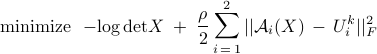
AMA consists of the following steps:
![begin{array}{rrcl} X-mathbf{minimization}~mathbf{step:} & ~~ X^{k+1} &!!mathrel{mathop:}=!!& {rm argmin}_{X} , {cal L}_0, ( X,, Z^k; , Y_1^k,, Y_2^k) [0.25cm] Z-mathbf{minimization}~mathbf{step:} & ~~ Z^{k+1} &!!mathrel{mathop:}=!!& {rm argmin}_{Z} , {cal L}_{rho}, ( X^{k+1},, Z; , Y_1^k,, Y_2^k) [0.25cm] Y-mathbf{update}~mathbf{step:} & ~~ Y_1^{k+1} &!!mathrel{mathop:}=!!& Y_1^k ,+, displaystyle{rho left( {cal A}_1 (X^{k+1}) , + , Z^{k+1} right)} [0.25cm] & ~~ Y_2^{k+1} &!!mathrel{mathop:}=!!& Y_2^k ,+, displaystyle{rho left( {cal A}_2 (X^{k+1}) , - , G right)} end{array}](eqs/1358873322516725525-130.png)
These terminate when the duality gap

and the primal residual

are sufficiently small, i.e.,  and
and  . In the -minimization step, AMA minimizes the Lagrangian
  with respect to . This step is followed by a -minimization step in which the augmented Lagrangian
  is minimized with respect to . Finally, the Lagrange multipliers, and , are updated based on the primal residuals with the step-size .
The -minimization step amounts to a matrix inversion and the -minimization step amounts to application of the soft-thresholding operator  on the singular values of a matrix:
![begin{array}{rcl} X^{k+1} &!!=!!& left( {cal A}_1^dagger (Y_1^k) ,+, {cal A}_2^dagger (Y_2^k) right)^{-1} [0.25cm] Z^{k+1} &!!=!!& {cal S}_tau left( - {cal A}_1 ( X^{k+1} ) , - , (1/rho)Y_1^k right), ~~~~ tau = gamma/rho [0.25cm] Y_1^{k+1} &!!=!!& {cal T}_{gamma} left(Y_1^k ,+, rho, {cal A}_1 (X^{k+1}) right) [0.25cm] Y_2^{k+1} &!!=!!& Y_2^k ,+, displaystyle{rho left( {cal A}_2 (X^{k+1}) , - , G right)} end{array}](eqs/6582258044759247696-130.png)
For Hermitian matrix  with singular value decomposition
  , and
, and  denote the singular value thresholding and saturation operators, respectively:
![begin{array}{rclrcl} {cal S}_tau (M) &!! mathrel{mathop:}= !!& U , {cal S}_tau (Sigma) ,U^*, & ~~~~ {cal S}_tau (Sigma) &!! = !!& {rm diag} left( left(sigma_i ,-, tau right)_+ right) [.25cm] {cal T}_tau (M) &!! mathrel{mathop:}= !!& U , {cal T}_tau (Sigma) ,U^*, & ~~~~ {cal T}_tau (Sigma) & !! = !! & {rm diag} left( min left( max( sigma_i, -, tau ), tau right) right) end{array}](eqs/7910724952940195208-130.png)
with  . The updates of Lagrange multipliers guarantee dual feasibility at each iteration, i.e.,
 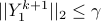 for all
  .
.
Alternating Direction Method of Multipliers (ADMM)
In contrast to AMA, ADMM minimizes the augmented Lagrangian in each step of the iterative procedure. In addition, ADMM does not have efficient step-size selection rules. Typically, either a constant step-size is selected or the step-size is adjusted to keep the norms of primal and dual residuals within a constant factor of one another Boyd, et al. ’11.
ADMM consists of the following steps:
![begin{array}{rrcl} X-mathbf{minimization}~mathbf{step:} & ~~ X^{k+1} &!!mathrel{mathop:}=!!& {rm argmin}_{X} , {cal L}_{rho}, ( X,, Z^k; , Y_1^k,, Y_2^k) [0.25cm] Z-mathbf{minimization}~mathbf{step:} & ~~ Z^{k+1} &!!mathrel{mathop:}=!!& {rm argmin}_{Z} , {cal L}_{rho}, ( X^{k+1},, Z; , Y_1^k,, Y_2^k) [0.25cm] Y-mathbf{update}~mathbf{step:} & ~~ Y_1^{k+1} &!!mathrel{mathop:}=!!& Y_1^k ,+, displaystyle{rho left( {cal A}_1 (X^{k+1}) , + , Z^{k+1} right)} [0.25cm] & ~~ Y_2^{k+1} &!!mathrel{mathop:}=!!& Y_2^k ,+, displaystyle{rho left( {cal A}_2 (X^{k+1}) , - , G right)} end{array}](eqs/8647659775536133319-130.png)
which terminate with similar stopping criteria to ADMM.
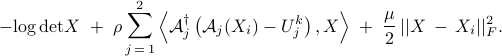
While the -minimization step is equivalent to that of AMA, the -update in ADMM is obtained by minimizing the augmented Lagrangian. This amounts to solving the following optimization problem
where 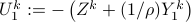 and
and 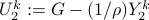 . From first order optimality conditions we have

Since  and
and  are not unitary operators, the -minimization step does not have an explicit solution. To solve this problem we use a proximal gradient method Parikh and Boyd ’13 to update . By linearizing the quadratic term around the current inner iterate
  and adding a quadratic penalty on the difference between and ,
  is obtained as the minimizer of
To ensure convergence of the proximal gradient method, the parameter  has to satisfy
 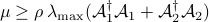 , where we use power iteration to compute the largest eigenvalue of the operator
 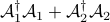 .
.
By taking the variation with respect to we arrive at the first order optimality condition
The solution to () can be iteratively computed as
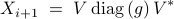
where the  th entry of the vector
  is given by
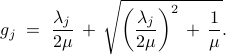
Here,  's are the eigenvalues of the matrix on the right-hand-side of () and
  is the matrix of the corresponding eigenvectors. As it is typically done in proximal gradient algorithms Parikh and Boyd ’13, starting with
  , we obtain
  by repeating inner iterations until the desired accuracy is reached.
Acknowledgements
This project is supported by the
National Science Foundation under Award CMMI 1363266
Air Force Office of Scientific Research under Award FA9550-16-1-0009
University of Minnesota Informatics Institute Transdisciplinary Faculty Fellowship